05 Probability

Julius-Maximilians-University Würzburg
Course: “Biostatistics”
Translational Neuroscience

Dr. Lea Hildebrandt

Probability

Probability theory: Branch of mathematics that deals with chance and uncertainty.

So far, we have summarized samples of data, but how do we draw inferences about the population?

–> to draw inferences (i.e., get reasonable estimates for the population), we need probability theory!

Probability = likelihood of some event (range from 0 = impossible to 1 = certain)

Sampling = next week

Is the mean of a sample equal to the mean of a population?

Probability = backbone of statistics, that’s why we cover it here as well!

(can be translated to percentages: * 100)

Probability Theory

Definitions:

• Experiment: Activity that produces outcome

• Sample space: Set of possible outcomes for an experiment

• Event: Subset of the sample space, an outcome

• Experiment: e.g. roll a die

• Sample space: six-sided die: {1,2,3,4,5,6}

• Event: e.g. 3

Hand out dice, coins etc to pairs.

Ask what Experiment, Sample Space and Event is in each case.

Probability Theory 2

Let’s say we have a variable \(X\) that contains \(N\) independent events:

\[ X = E_1, E_2, …, E_n \]

The probability of a certain event (event \(i\)) is then formally written as:

\[ P(X = E_i) \]

Formal features of probability theory:

1. Probability can’t be negative.

2. The total probability of outcomes in the sample space is 1.

3. The probability of any individual event can’t be greater than 1.

What is N and E’s in dice/coins case?

Do the 3 features make sense in their own example? Height e.g. is difficult

Determine Probabilities

How would you determine probabilities? E.g. how likely is it that you roll a 6 or toss head? (Think about your own example!)

• Personal belief (not very scientific!)

• Empirical frequency

  • Law of large numbers

• Classical probability

personal belief: What would have been? Which vaccination is best (opinion)

empirical: count events from the past, divide by possible events (rain days from all days)
–> which year(s)? The more data, the better

Law of large numbers: The more times you repeat an experiment, the less likely you get extreme values.

Classical Probability

Rules of probability

1. What is the probability of an event not happening? (E.g. not rolling a 6)
   1. Subtraction: Probability of some event (A) not happening = 1- probability that it happens:
      • \(P(\neg A) = 1 - P(A)\)
2. What is the probability of two events happening together, i.e. rolling a 3 and a 4 or tossing two heads?
   1. Intersection: The probability of a conjoint event/that both A and B will occur (\(\cap\)):
      • \(P(A \cap B) = P(A) * P(B)\) (if A and B are independent!)
3. What is the probability of either of two events occuring, e.g. rolling a 3 or a 4?
   1. Addition: Probability of either of two events occurring (\(\cup\)):

      • \(P(A \cup B) = P(A) + P(B) - P(A \cap B)\)

      • We add both but subtract the intersection, prevents us from counting intersection twice!

Ask for every point how they would try to figure it out with dice/coins

\(\neg A\) = “not A”, derives from Axioms above: Sum must be 1

\(\cap\) = or; \(\cup\) = and

addition: difference 1 vs. 2 dice!

Classical Probability 2

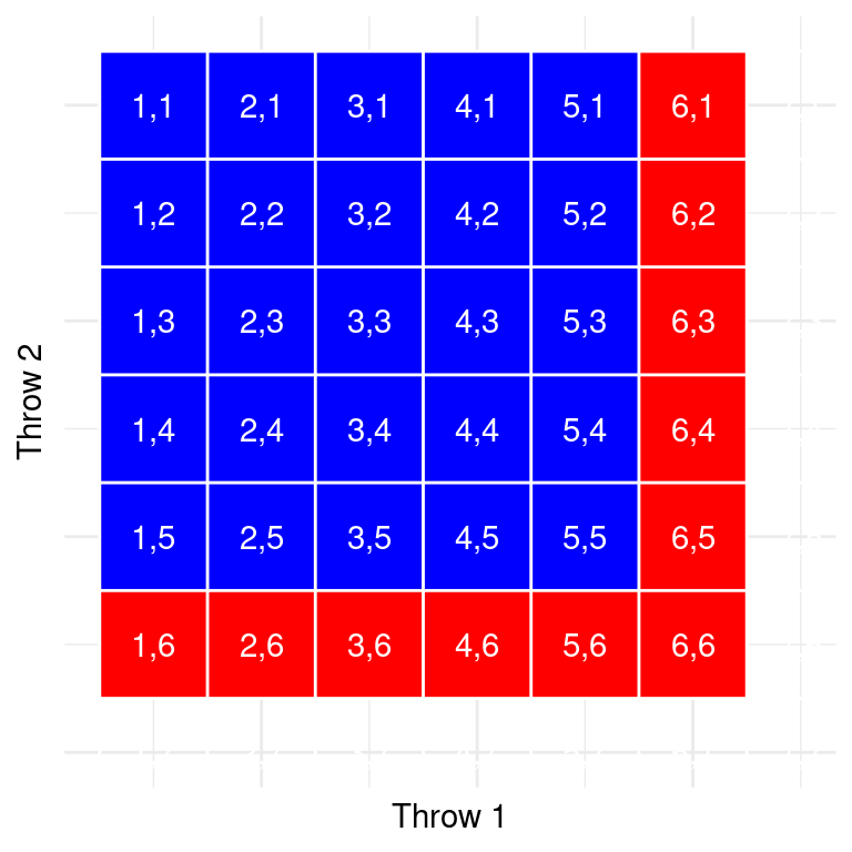
Probability of getting at least one 6 within two dice rolls: 11x success out of 36 possibilities: \(\frac{11}{36} = 30.1\%\)

Each cell in this matrix represents an outcome of throws of two dice (rows = one die, columns = other die). Cells in red represent the cells with a six.

Don’t count 6,6 twice!

For example, go to book

Probability is important for statistics, so it is necessary to go through the rules once

–> necessary to draw inferences from data! How representative are data for population?

Conditional Probability

How likely is an event given that another event has occurred?

\[P(A|B) = \frac{P(A \cap B)}{P(B)}\]

“The conditional probability of A given B is the joint probability divided by the overall probability of B”.

Example: The conditional probability of being infected with Covid-19, given a positive test result (it could be a false positive!). This will be illustrated in more detail in conjunction with Bayes’ Rule.

How likely to roll a 6 if previously a 5? NO, independent events!

How likely is it that you pass the class if you have taken the course?

Probability that both things are true given that the one being conditioned upon is true

Independence

Starting point: \[P(A|B) = \frac{P(A \cap B)}{P(B)}\] For independence: \[ P(A \cap B) = P(A) * P(B) \] This means: \[P(A|B) = \frac{P(A)*P(B)}{P(B)} = P(A)\]

=> Independence = Knowing the value of one variable doesn’t tell us anything about the value of the other

But if the two variables are dependent, the conditional probability \(P(A|B)\) will differ from the overall probability \(P(A)\).

Comparing conditional and overall prob might be helpful to determine whether variables are independent.

Ex: physical activity and mental health.

Use conditional probability in most cases!

Exercises

1. There have been 10 parties so far. Anna has gone to 5 of them, Barbara to 8. How likely do you expect each Anna and Barbara to go to the next party?

\[ P(A) = \frac{5}{10} = 50\%; P(B) = \frac{8}{10} = 80\% \]

2. Out of the 10 parties, to how many have both Anna and Barbara been under the assumption that they went to parties independently?

\[ P(A \cap B) = P(A) * P(B) = .5 * .8 = 40\% \]

3. You learn that, in fact, Anna and Barbara have both been present at 5 parties. From this information, would you expect that Anna and Barbara are a) friends, b) don’t like each other, c) neither?

Anna and Barbara have both been present at 5 parties but should have been only at 4 given independence. Thus, they were there together more often than “by chance”, indicating that they may have arranged to go together. Hence, they may be friends. (If this increment from 4 to 5 parties is also statistically significant will be answered in the upcoming lectures.)

4. You are late to the 11th party - everyone else is already there. You enter the apartment and see Barbara. How likely do you think Anna will also be there?

\[ P(A|B) = \frac{P(A \cap B)}{P(B)} = \frac{50\%}{80\%} = 62.5\% \] 62.5% is not huge but bigger than the prior probability to find Anna at a party of \(P(A) = 50\%\)!

5. You are late to the 11th party - everyone else is already there. You enter the apartment and see Anna. How likely do you think Barbara will also be there?

\[ P(B|A) = \frac{P(A \cap B)}{P(A)} = \frac{50\%}{50\%} = 100\% \] We have never seen Anna at a party without Barbara (both \(P(A)\) and \(P(A \cap B)\) are 50%). Thus, we are pretty sure to find Barbara once we see Anna (unless the pattern changes).

3. Imagine Anna and Barbara hate each other such they would never (or very unlikely) go to the same party. Then, \(P(A \cap B) < P(A) * P(B)\). If they like each other, \(P(A \cap B) > P(A) * P(B)\).

Bayes’ Rule

Often we know \(P(B|A)\) but really want to know \(P(A|B)\)!

Example: From the test manual, we know the probability of getting a positive Covid test when we actually have Covid, \(P(positive|Covid)\). But we usually want to know the probability of having Covid once we tested positive, \(P(Covid|positive)\).

This reversed conditional probability can be calculated using Bayes’ Rule:

\[P(A|B) = \frac{P(A) * P(B|A)}{P(B)}\]

If we have two outcomes, we can expand using:

\[P(B) = P(A \cap B) + P(\neg A \cap B) = P(A) * P(B|A) + P(\neg A) * P(B|\neg A)\]

Updated Bayes’ Rule:

\[P(A|B) = \frac{P(A)*P(B|A)}{P(A)*P(B|A) + P(\neg A)*P(B|\neg A)}\]

Bayes’ Rule 2

Example: Let’s try to find out:

\[P(Covid|positive) = \frac{P(Covid) * P(positive|Covid)}{P(positive)}\]

Tests can’t be 100% correct, there are always false positives and false negatives. But let’s say the sensitivity of the test \(P(positive|Covid)\) is 95% and the specificity \(P(negative|healthy)\) is 75%.

We’d also need the prevalence of Covid, \(P(Covid)\), which is (let’s say) 10%.

Finally, we plug in \(P(pos) = P(Covid) * P(pos|Covid) + P(healthy) * P(pos|healthy)\). So that would be

\[P(positive) = .1 * .95 * + (1-.1) * (1-.95) = .14\]

Bringing it together, we get:

\[P(Covid|positive) = \frac{.1 * .95}{.14} = .679\]

If we test positive, we’d thus are actually infected with a probability of 67.9%!

(But before, we only had 10%, i.e. \(P(Covid)\))

Learning from Data

The terms in Bayes’ Rule have some specific names:

\[P(Covid|positive) = \frac{P(Covid) * P(positive|Covid)}{P(positive)}\]

The prevalence \(P(Covid)\) in our example is also called the prior probability (before we have any further information, e.g. the test result).

After we collected new evidence (= test result), we have the likelihood: \(P(positive|Covid)\), which is the sensitivity of the test.

\(P(positive)\) is the marginal likelihood (overall likelihood positive tests across infected and healthy individuals).

Finally, \(P(Covid|test)\) is the posterior probability (after accounting for the new observation).

\[ P(B|A) = \frac{P(A|B)}{P(A)} * P(B) \]

\(P(A|B)/P(A)\) = how likely the data are given B relative to overall marginal likelihood (how likely a pos rest if Covid relative to how likely it is to have a pos. test in general)

\(P(B)\) = how likely we thought it was to have Covid before we knew the test result

Sum Up

Models and probability are central to statistics, as we will see.

There are two intepretations of probability: Frequentist and Bayesian.
Frequentists interpret probability as the long-run frequencies (e.g. how many people end up getting Covid).

Bayesians interpret probability as a degree of belief. How likely is it to catch Covid if you go out now? Based on beliefs and knowledge.

Freq: Difficult to wrap ones’ head around if an event occurs only once.

Bayes: Bit more subjective

Probability Distributions

We already covered classic probability theory, including conditional probability.

Today, we will go more into depth about different probability distributions.

Probability distribution = probability of all possible outcomes in an experiment.

Helps us answer questions like: How likely is it that event X occurs/we find specific value of X? (\(P(X = x_i)\))

Cumulative Probability Distribution

–> how likely is it to find a value that is as extreme or larger (or as small or smaller!)? (\(P(X \geq x_i)\))

A probability distribution is similar to a frequency distribution: The difference is that the probability distribution reflects the theory and the frequency distribution the observed data (i.e., frequencies are used to approximate probabilities)

Simulations can be used to get (an approximation of) a probability distribution!
We don’t have to conduct an experiment, e.g., tossing a coin 100x, but can rather simulate it using R!

freq dist: How many times did an event occur? (e.g. flipping a coin, getting tails)

prob dist: How many times should it have occurred? 50% but also realistic lower and higher values!

The Uniform Distribution

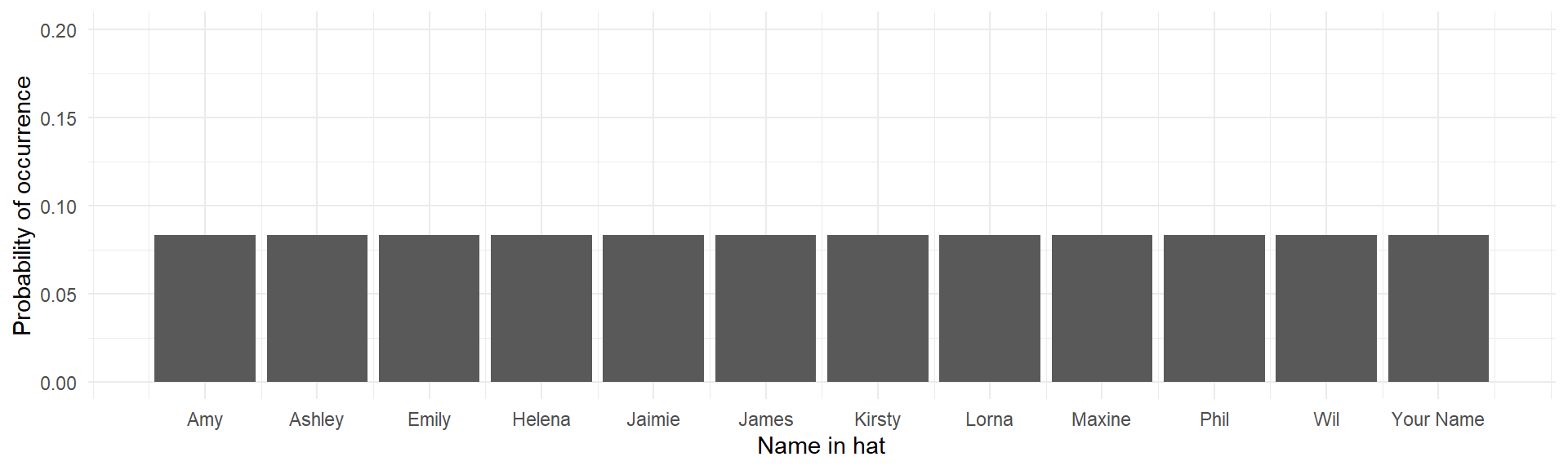
In a uniform distribution, each possible outcome has an equal chance of occurring.

If we have a hat with 12 paper slips with names, each name has an equal chance (\(p = \frac{1}{12} \approx .08\)) of being drawn:

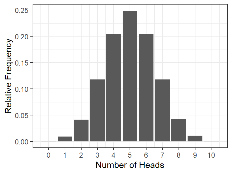
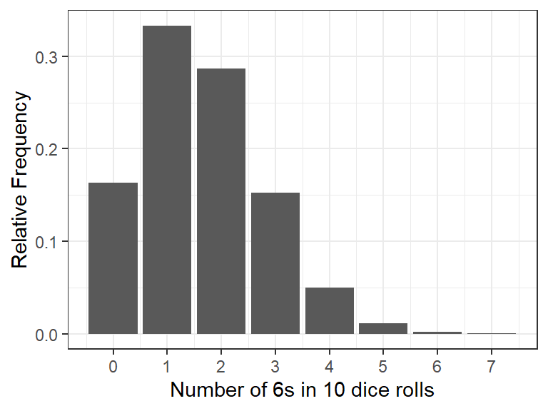
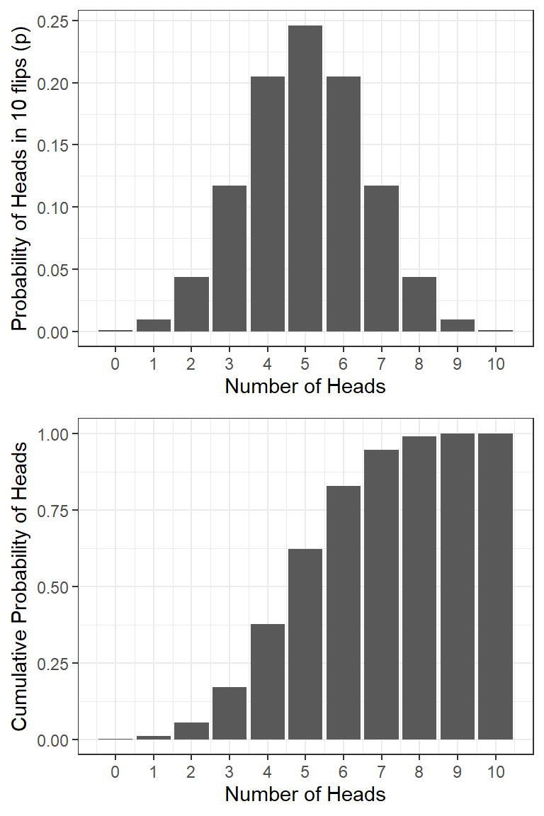
The Binomial Distribution

The binomial (“two categories”) distribution is used for discrete data with two possible outcomes (e.g., flipping a coin). It models the number of successes being observed (e.g., heads), given the probability of success (0.5 for fair coins) and the number of observations (flips of a coin, e.g., 10).

How many heads (successes) should we expect and with what probability?

We can simulate 10 coin flips (or dice) each 10.000 times and count the number of heads (out of the 10). We can use this distribution to work out the probability of different outcomes, e.g., getting at least 3 heads (or 6s) out of 10 tosses (dice rolls).

success: whatever you want, also an “artificial” dichotomization like “roll a 6” vs. “roll no 6”

add up probabilities >=3 or 1 - P(X <= 2)

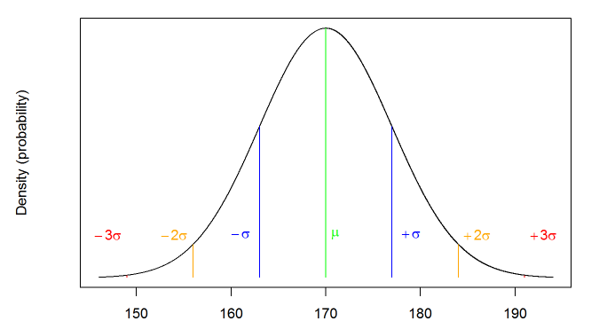
The Normal Distribution

The normal distribution is very common in statistics (i.e., in the real world). It (roughly) reflects the probability of any value occurring for a continuous variable, such as height.

Normal distribution of height

The normal distribution is always symmetrical
=> equal probability of observations above and below the mean.
=> the mean, median, and mode are all equal!

Normal Distribution 2

We can also use simulations to approximate a normal distribution. This simulation shows that increasing the sample size will get closer to a normal distribution:

A simulation of an experiment collecting height data from 5000 participants.

R

Open RStudio and load your Biostats R project. Create a new script called Probability.R.

Distributions

We are starting with exercises about the three distributions we just got know: uniform, binomial, and normal distribution.

Using the Uniform Distribution

We can use runif for a uniform distribution of continuous (numerical) values or
sample for a uniform distribution of discrete (numerical or text) values.

1. Draw a random decimal number between 0 and 1
2. Draw 100 random decimal numbers between 0 and 10 and calculate their mean.
3. Draw 50 random integer numbers between 1 and 10 and calculate their mean.
4. Draw who may have the first turn during board game night: Anna, Barbara, Christina, or Dana.
5. Produce a random order of all the names of Anna, Barbara, Christina, and Dana.

#1
runif(n=1) #default parameters are already set to min=0 and max=1

[1] 0.5325043

#2
runif(n=100, max=10) %>% mean()

[1] 5.37693

#3
sample(1:10, size=50, replace=T) %>% mean()

[1] 5.82

#4
sample(c("Anna", "Barbara", "Christina", "Dana"), size=1)

[1] "Dana"

#5
sample(c("Anna", "Barbara", "Christina", "Dana")) #by default, sample draws all elements in random order

[1] "Barbara"   "Christina" "Anna"      "Dana"     

Using the Binomial Distribution

• dbinom(): the density distribution gives you the probability of exactly \(x_i\) successes given the number of trials and the probability of success on a single trial: \(P(X = x_i)\) (e.g., what’s the probability of flipping 8/10 heads with a fair coin?)

• pbinom(): the (cumulative) probability distribution gives you the cumulative probability of getting a maximum of \(x_i\) successes: \(P(X \le x_i)\) (e.g., getting 5 or fewer heads out of 10 flips).

• qbinom(): the quantile function gives you the number of success (x-axis) corresponding to a given cumulative probability: \(X(P = P_i)\) (e.g., A maximum of how many heads do you have to expect if you want at least an event probability of 25%?). This is the inverse function of pbinom().

Note: Be aware of the difference between success probability \(p\), the probability of the density distribution \(P(X = x_i)\), and the probability of the cumulative probability distribution \(P(X \le x_i)\)

1. What’s the probability of getting exactly 5 heads on 10 flips?
2. What’s the probability of getting 0 to 2 heads on 10 flips?
3. What’s the probability of getting at least 8 heads on 10 flips?

Using the Binomial Distribution 2

Now in R:

1. What’s the probability of getting exactly 5 heads on 10 flips?
2. What’s the probability of getting 0 to 2 heads on 10 flips?
3. What’s the probability of getting at least 8 heads on 10 flips?

#1
dbinom(x = 5, size = 10, prob = 0.5)

[1] 0.2460938

#2 (indirect way)
dbinom(x = 0:2, size=10, prob=0.5) %>% sum()

[1] 0.0546875

#2 (direct way)
pbinom(q = 2, size = 10, prob = 0.5) #P(X <= q)

[1] 0.0546875

#3 (careful: minus 1)
pbinom(q = 8-1, size = 10, prob = 0.5, lower.tail = F) #P(X > q) = 1 - P(X <= q)

[1] 0.0546875

Note: The binomial distribution is only symmetrical for \(p = 50\%\).
That’s why “a maximum of 2 heads” (0, 1, or 2) has the same probability as “at least 8 heads” (8, 9, or 10).

• x: the number of ‘heads’ of which we want to know the probability.

• size: the number of trials (flips) we are simulating; in this case, 10 flips.

• prob: the probability of ‘heads’ on one trial. 50% far a fair coin.

Using the Binomial Distribution 3

Now let’s use the quantile function qbinom()!

Imagine a friend wants to bet you on tossing a coin and bets that it will be tails. You suspect she has a coin that is not fair and it will be more likely that it turns up as tails.

Your friend agrees that you can toss the coin 10 times to test it before you have to give your bet.
you want to find out whether the coin is fair and ask yourself: What is the minimum number of heads that is acceptable if it is fair?

We choose a probability so low that it is unlikely to get a result lower than that if the coin was fair. We will use a typical value for statistical significance: 0.05 (or in 5% of cases we will find a lower value by chance if the coin was fair).

qbinom(p = .05, size = 10, prob = .5)

[1] 2

In this case, the probability of success is now called prob because p is now used for the probability cut-off we want to set. This is unnecessarily confusing :(

If we run the code, we get a value of 2. This means that 2 heads is the first time that the cumulative probability function reaches at least 5% . Thus, if we get less than two heads out of the ten tosses, we could conclude that the coin is likely biased (there is only a 5% chance that this would happen if the coin was fair). You would probably not bet with your friend!

Note: This is a bad way to test the fairness of a coin (it’s just for illustration of qbinom)! Rather demand that you win at tails (if the coin is fair, your friend shouldn’t mind).

Using the Normal Distribution

For every probability distribution, R provides similar functions starting with d, p, or q. For the normal distribution, those are:

• dnorm(): density function, for calculating the density (not probability!) of a specific value. Only useful for plotting.

• pnorm(): cumulative probability or distribution function, for calculating the probability of getting at least (or at most) a specific value.

• qnorm(): quantile function, for calculating the specific value associated with a given cumulative probability.

For the next activities, we will use means and SDs of height from the Scottish Health Survey (2008).

Using the Normal Distribution 2

Calculate the probability of meeting a Scottish woman who is as tall or taller than the average Scottish man.

Which function would you use?

Hint: You want to know how likely it is that you get a value as extreme or extremer than a specific value (the average height of men) within the distribution for women.

What we know:

• average female height = 163.8, SD = 6.931

• average male height = 176.2, SD = 6.748

• We want to know “at least as tall as”

We need the pnorm() function. Fill in the values instead of the NULLs.

pnorm(q = NULL, mean = NULL, sd = NULL, lower.tail = NULL)

pnorm(q = 176.2, mean = 163.8, sd = 6.931, lower.tail = FALSE)

[1] 0.03680228

Note: For continuous distributions, we don’t have to distinguish between “taller than” and “at least as tall”. \(P(X \le x_i) = P(X < x_i)\)! (Because the probability of one specific value like 176.2000000 m is exactly 0)

Also note: The SD of the distribution of males is not relevant for this question.

Don’t do this:

pnorm(q = 176.2, mean = 163.8, sd = 6.931, lower.tail = F) + 
  dnorm(x = 176.2, mean = 163.8, sd = 6.931)

[1] 0.04841892

You cannot add a probability and a density together! Just pnorm(q = 176.2, mean = 163.8, sd = 6.931, lower.tail = F) is the correct answer!

When we say “What’s the probability of a woman being 1.80 m tall?”, we actually mean: “What’s the probability of a person being between 1.795 and 1.805 m tall?” (since height is usually measured within steps of 1 cm). We can calculate this, e.g. for Scottish women, using: pnorm(q = 180 + c(-.5, .5), mean = 163.8, sd = 6.931) %>% diff() = 0.3%

Using the Normal Distribution 3

Fiona is a very tall Scottish woman (181.12 cm) who will only date men who are as tall or taller than her. What is the probability of Fiona finding a taller man?

What we know:

• average female height = 163.8, SD = 6.931

• average male height = 176.2, SD = 6.748

• We want to know “tall or taller”

• Fiona’s height = 181.12

pnorm(q = 181.12, mean = 176.2, sd = 6.748, lower.tail = FALSE)

[1] 0.2329687

Conclusion: Fiona shrinks her dating pool to roughly a quarter and may thus consider abandoning beauty standards imposed by society. (Same advice for men, of course)

How tall would a Scottish man have to be in order to be in the tallest 5% of the height distribution for Scottish men?

qnorm(p = .05, mean = 176.2, sd = 6.748, lower.tail = FALSE)

[1] 187.2995

Thanks!

Learning objectives:

• Understand different concepts of probability:

  • joint and conditional probability

  • statistical independence

  • Bayes’ Theorem

  • probability distributions

• Understand and use different probability distributions in R

Next:

• Sampling and resampling/simulations