Dr. Mario Reutter (slides adapted from Dr. Lea Hildebrandt)
Probability
Probability theory: branch of mathematics that deals with chance and uncertainty.
So far, we have summarized samples of data, but how do we draw inferences about the population? Is the mean of a sample equal to the mean of the population?
--> to draw inferences (i.e., get reasonable estimates for the population), we need probability theory!
Probability = likelihood of some event (range from 0 = impossible to 1 = certain)
(can be translated to percentages: * 100)
Probability Theory
Definitions:
Experiment: Activity that produces outcome (e.g. roll a die)
Sample space: Set of possible outcomes for an experment (six-sided die: {1,2,3,4,5,6})
Event: Subset of the sample space, an outcome
Probability Theory 2
Let’s say we have a variable \(X\) that contains \(N\) independent events:
\[
X = E_1, E_2, …, E_n
\]
The probability of a certain event (event \(i\)) is then formally written as:
\[
P(X = E_i) \]
Formal features of probability theory:
Probability can’t be negative.
The total probability of outcomes in the sample space is 1.
The probability of any individual event can’t be greater than 1.
Determine Probabilities
Personal belief (not very scientific!)
Empirical frequency
Law of large numbers
Classical probability
Classical Probability
Rules of probability
Subtraction: Probability of some event (A) not happening = 1- probability that it happens:
\(P(\neg A) = 1 - P(A)\)
Intersection: The probability of a conjoint event/that both A and B will occur (\(\cap\)):
\(P(A \cap B) = P(A) * P(B)\) (if A and B are independent!)
Addition: Probability of either of two events occurring (\(\cup\)):
\(P(A \cup B) = P(A) + P(B) - P(A \cap B)\)
We add both but subtract the intersection, prevents us from counting intersection twice!
Classical Probability 2
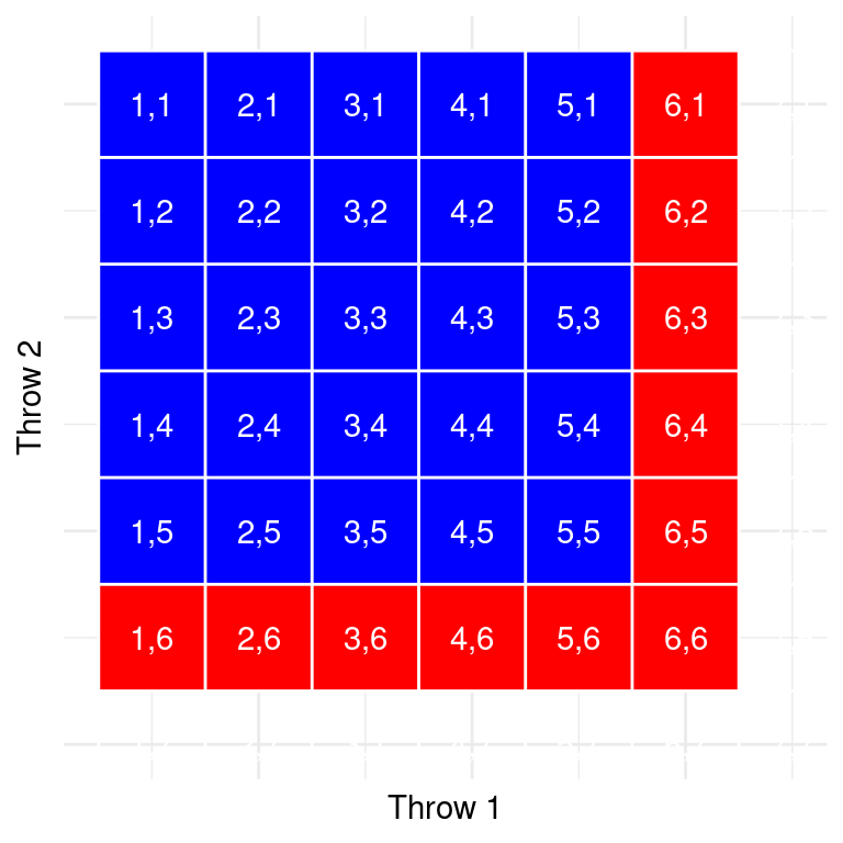
Probability of getting at least one 6 within two dice rolls: 11x success out of 36 possibilities: \(\frac{11}{36} = 30.1\%\)
Each cell in this matrix represents an outcome of throws of two dice (rows = one die, columns = other die). Cells in red represent the cells with a six.
Conditional Probability
How likely is an event given that another event has occurred?
\[P(A|B) = \frac{P(A \cap B)}{P(B)}\]
“The conditional probability of A given B is the joint probability divided by the overall probability of B”.
Example: The conditional probability of being infected with Covid-19 given a positive test result (it could be a false positive!). This will be illustrated in more detail in conjunction with Bayes’ Rule.
Independence
Starting point: \[P(A|B) = \frac{P(A \cap B)}{P(B)}\] For independence: \[ P(A \cap B) = P(A) * P(B) \] This means: \[P(A|B) = \frac{P(A)*P(B)}{P(B)} = P(A)\]
=> Independence = Knowing the value of one variable doesn’t tell us anything about the value of the other
But if the two variables are dependent, the conditional probability \(P(A|B)\) will differ from the overall probability \(P(A)\).
Exercises
There have been 10 parties so far. Anna has gone to 5 of them, Barbara to 8. How likely do you expect each Anna and Barbara to go to the next party?
Out of the 10 parties, to how many have both Anna and Barbara been under the assumption that they went to parties independently?
\[ P(A \cap B) = P(A) * P(B) = .5 * .8 = 40\% \]
You learn that, in fact, Anna and Barbara have both been present at 5 parties. From this information, would you expect that Anna and Barbara are a) friends, b) don’t like each other, c) neither?
Anna and Barbara have both been present at 5 parties but should have been only at 4 given independence. Thus, they were there together more often than “by chance”, indicating that they may have arranged to go together. Hence, they may be friends. (If this increment from 4 to 5 parties is also statistically significant will be answered in the upcoming lectures.)
You are late to the 11th party - everyone else is already there. You enter the apartment and see Barbara. How likely do you think Anna will also be there?
\[ P(A|B) = \frac{P(A \cap B)}{P(B)} = \frac{50\%}{80\%} = 62.5\% \] 62.5% is not huge but bigger than the prior probability to find Anna at a party of \(P(A) = 50\%\)!
You are late to the 11th party - everyone else is already there. You enter the apartment and see Anna. How likely do you think Barbara will also be there?
\[ P(B|A) = \frac{P(A \cap B)}{P(A)} = \frac{50\%}{50\%} = 100\% \] We have never seen Anna at a party without Barbara (both \(P(A)\) and \(P(A \cap B)\) are 50%). Thus, we are pretty sure to find Barbara once we see Anna (unless the pattern changes).
Bayes’ Rule
Often we know \(P(B|A)\) but really want to know \(P(A|B)\)!
Example: From the test manual, we know the probability of getting a positive Covid test when we actually have Covid, \(P(positive|Covid)\). But we usually want to know the probability of having Covid once we tested positive, \(P(Covid|positive)\).
This reversed conditional probability can be calculated using Bayes’ Rule:
\[P(A|B) = \frac{P(A) * P(B|A)}{P(B)}\]
If we have two outcomes, we can expand using:
\[P(B) = P(A \cap B) + P(\neg A \cap B) = P(A) * P(B|A) + P(\neg A) * P(B|\neg A)\]
Tests can’t be 100% correct, there are always false positives and false negatives. But let’s say the sensitivity of the test \(P(positive|Covid)\) is 95% and the specificity\(P(negative|healthy)\) is 75%.
We’d also need the prevalence of Covid, \(P(Covid)\), which is (let’s say) 10%.
Finally, we plug in \(P(pos) = P(Covid) * P(pos|Covid) + P(healthy) * P(pos|healthy)\). So that would be
The prevalence \(P(Covid)\) in our example is also called the prior probability (before we have any further information, e.g. the test result).
After we collected new evidence (= test result), we have the likelihood: \(P(positive|Covid)\), which is the sensitivity of the test.
\(P(positive)\) is the marginal likelihood (overall likelihood positive tests across infected and healthy individuals).
Finally, \(P(Covid|test)\) is the posterior probability (after accounting for the new observation).
Probability Distributions
Probability distribution = probability of all possible outcomes in an experiment.
Helps us answer questions like: How likely is it that event X occurs/we find specific value of X? (\(P(X = x_i)\))
Cumulative Probability Distribution
--> how likely is it to find a value that is as extreme or larger (or as small or smaller!)? (\(P(X \geq x_i)\))
Sum Up
Models and probability are central to statistics, as we will see.
There are two intepretations of probability: Frequentist and Bayesian.
Frequentists interpret probability as the long-run frequencies (e.g. how many people end up getting Covid).
Bayesians interpret probability as a degree of belief. How likely is it to catch Covid if you go out now? Based on beliefs and knowledge.
Sampling
We have already mentioned the difference between the whole population and our sample. To be able to draw inferences from a relatively small sample to a population is one of the core ideas of statistics.
Why do we sample?
Time: It’s often impossible to measure whole population.
A subset (sample) might be sufficient to estimate a value of interest (diminishing marginal returns).
How Do We Sample?
The sample needs to be representative of the entire population, that’s why it’s critical how we select the individuals.
Think about examples of non-representative samples!
Representative: Every member of the population has an equal chance of being selected.
If non-representative: sample statistic is biased, its value is different from the true population value (parameter).
(But talking about bias is mostly a theoretical discussion: Usually we of course don’t know the population parameter and thus cannot compare our estimate with it! Otherwise we wouldn’t need to sample.)
Different Ways of Sampling
without replacement: Once a member of the population is sampled, they are not eligible to be sampled again. This is the most common variant of sampling.
with replacement: After a member of the population has been sampled, they are put back into the pool and could potentially be sampled again. This usually happens out of accident or by necessity (cf. Bootstrapping)
Sampling Error
It is likely that our sample statistic differs slightly from the population parameter. This is called the sampling error.
If we collect multiple samples, the sample statistic will always differ slightly. If we combine all those sample statistics, we can approximate the sampling distribution.
Of course, we want to minimize the sampling error and get a good estimate of the population parameter!
Example Sampling Distribution
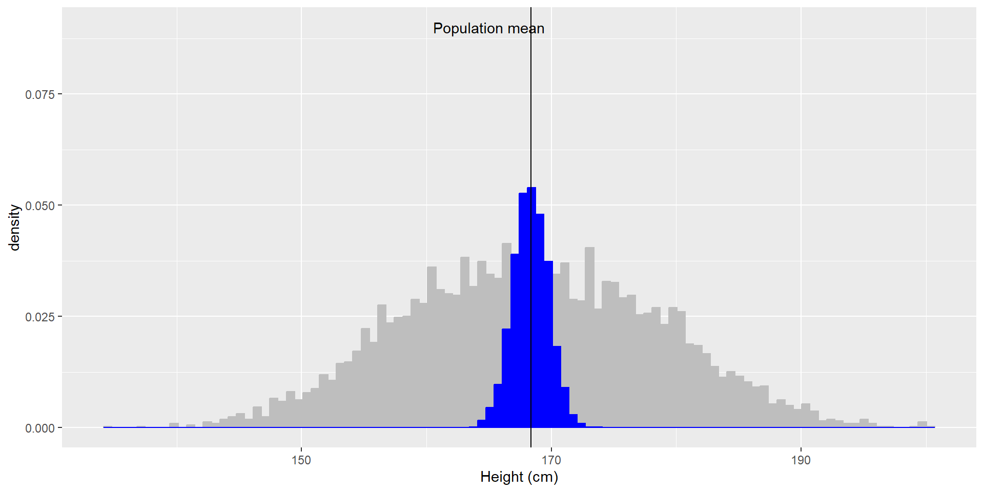
Let’s use the NHANES dataset again and let’s assume it is the entire population. We can calculate the mean (\(\mu = 168.35\)) and standard deviation (\(\sigma = 10.16\)) as the population parameters. If we repeatedly sample 50 individuals, we get this:
sampleMean
sampleSD
169.590
9.583388
168.764
10.847642
169.892
9.543752
170.288
10.837005
169.330
10.270072
The sample means and SDs are similar, but not exactly equal to the population parameters.
If we sample 5000 times (50 individuals each), we can see that the average of these 5000 sample means (depicted in blue) is similar to the population mean!
Average sample mean across 5000 sample: \(\hat{X} = 168.3463\).
Standard Error of the Mean
In the example on the last slide, the means were all pretty close to each other, i.e. the blue distribution was very narrow and the variance small (compared to the grey distribution). This is an inherent statistical property of sample means: By averaging several individual values, thus aggregating them into a sample (here with \(n = 50\)), we reduce the variability of the sampling distribution.
We can quantify this variability of the sample mean with the standard error of the mean (SEM).
\[SEM = \frac{\hat{\sigma}}{\sqrt{n}}\]
This formula needs two values: the population variability \(\sigma\) (or sample SD \(\hat{\sigma}\) as approximation) and the size of our sample \(n\).
We can only control our sample size, thus if we want a better estimate, we can increase sample size!
A sample of \(n = 50\) already decreases the population variability by a factor of \(\sqrt{50} = 7.1\) !
The Central Limit Theorem
The Central Limit Theorem (CLT) is a fundamental (and often misunderstood) concept of statistics.
CLT: With larger sample sizes, the sampling distribution of sample means (i.e., the blue distribution from before) will become more and more normally distributed*, even if the population distribution is not (i.e., the grey distribution from before)!
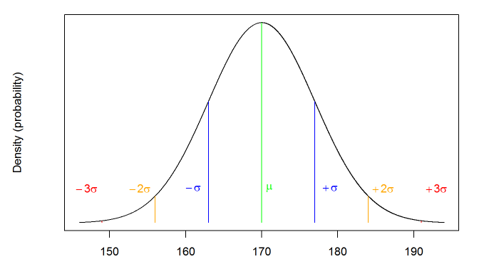
Normal Distribution of Height
Note: Means approximate a normal distribution, irrespective of the distribution from which the data stem. This is because the sampling error between the sampling mean \(\hat{\mu}\) and the population mean \(\mu\) follows a normal distribution.
CLT in Action
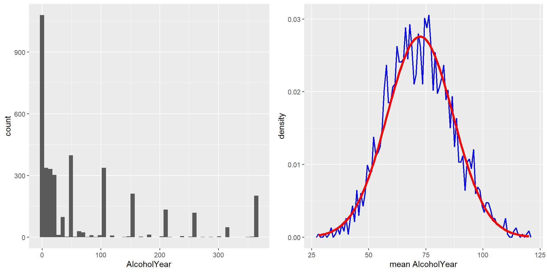
On the left you can see a highly skewed distribution of alcohol consumption per year (from the NHANES dataset). If we repeatedly draw samples of size 50 from the datset and take the mean, we get the right distribution of sample means - which looks a lot more “normal” (normal distribution is added in red)!
The CLT is important because it allows us to safely assume that the sampling distribution of the mean will be normal in most cases, which is a necessary prerequisite for many statistical techniques.
Resampling and Simulation
Monte Carlo Simulation
With the increasing use of computers, simulations have become an essential part of modern statistics. Monte Carlo simulations are the most common ones in statistics.
There are four steps to performing a Monte Carlo simulation:
Define a domain of possible values.
Generate random numbers within that domain from a probability distribution.
Perform a computation using the random numbers.
Combine the results across many repetitions.
Randomness in Statistics
Random = unpredictable.
For a Monte Carlo simulation, we need pseudo-random* numbers, which are generated by a computer algorithm.
We can simply generate (pseudo-)random numbers from different distributions with R, e.g. with rnorm() to draw (pseudo-)random numbers from a normal distribution:
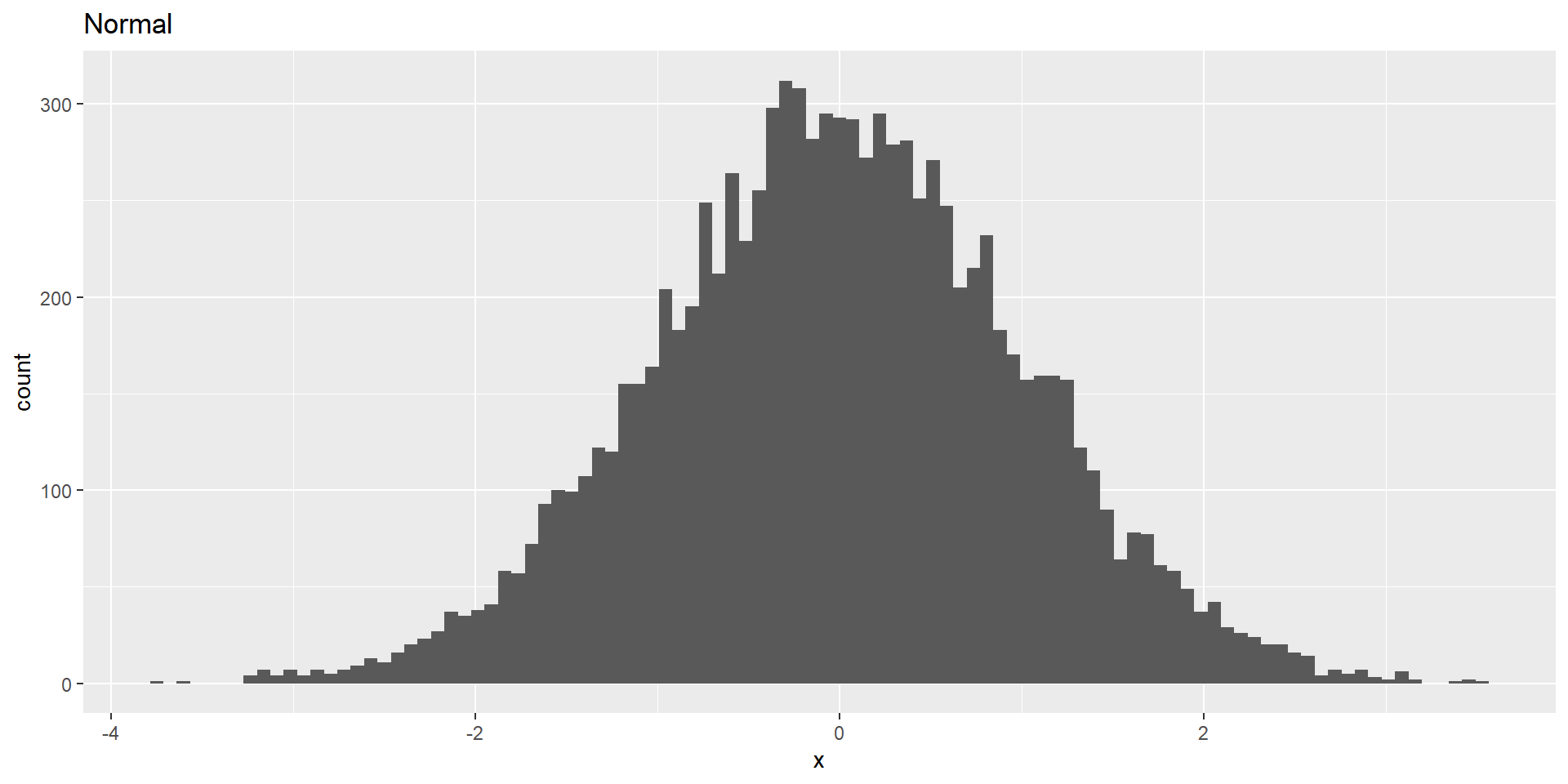
# Draw 10000 random numbers of a normal distribution with mean=0, sd=1rand_num <-rnorm(n=10000, mean=0, sd=1)# Plot the random numbers and verify that they make up a normal distributiontibble(x = rand_num) %>%ggplot(aes(x)) +geom_histogram(bins =100) +labs(title ="Normal")
Each time, we generate random numbers, these will differ slightly.
But we can also generate the exact same set of random numbers (which will be helpful to reproduce results!) by setting the random seed to a specific value such as 123: set.seed(123).
Using Monte Carlo Simulations
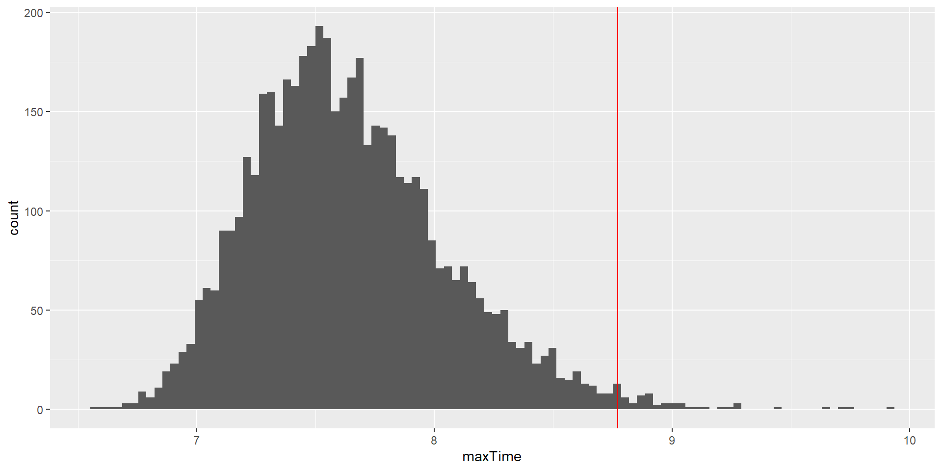
Example: Let’s try to find out how much time we should allow for a short in-class quiz.
We pretend to know the distribution of completion times is normal, with mean = 5 min and SD = 1 min.
How long does the test period need to be so that we can expect ALL students (n = 150) to finish in 99% of the quizzes?
To answer this question, we need the distribution of the longest finishing time.
What we will do is to simulate finishing times for a great number of quizzes and take the maximum of each (the longest finishing time). We can then look at the distribution of maximum finishing times and see where the 99% quantile is.
This value is the amount of time that we should allow - given our assumptions!!
Using Monte Carlo Simulations 2
Let’s repeat the steps of the simulation by going through the four steps mentioned before:
Define a domain of possible values.
--> Our assumptions: The values would come from a normal distribution with \(n = 150\), \(mean = 5\), and \(SD = 1\).
Generate random numbers within that domain from a probability distribution.
rand_num <-rnorm(n =150, mean =5, sd =1)
Perform a computation using the random numbers.
max_rand_num <-max(rand_num) #time of slowest student
Using Monte Carlo Simulations 3
Combine the results across many repetitions.
nrep <-5000#number of repetitions# initialize an empty matrix to fill in the max values latermax_rand_num <-matrix(data =NA, nrow = nrep, ncol=1)# use a for-loop to repeat resampling nrep times!for (i in1:nrep) { rand_num <-rnorm(n =150, mean =5, sd =1) max_rand_num[i, 1] <-max(rand_num)}# get the cutoff (99%) of the distribution of max valuescutoff <-quantile(max_rand_num, 0.99)print(cutoff)
     99%
8.846554
Using Monte Carlo Simulations 4
This shows that the 99th percentile of the finishing time distribution falls at 8.7723092 minutes, meaning that if we were to give that much time for the quiz, then we expect that in 99% of quizzes, every student would finish.
The Bootstrap
We can use simulations to demonstrate statistical principles (like we just did) but also to answer statistical questions.
The bootstrap is a simulation technique that allows us to quantify our uncertainty of estimates!
We repeatedly sample with replacement from an actual dataset.
We compute a statistic of interest for each sample.
We get the distribution of those statistics and use it as our sampling distribution.
Bootstrap Example
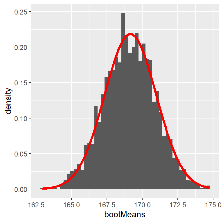
Let’s use the bootstrap to estimate the sampling distribution of the mean heights of the NHANES dataset. We can then compare the result to the SEM (=uncertainty of the mean) that we discussed earlier.
# perform the bootstrap to compute SEM and compare to parametric methodnRuns <-2500sampleSize <-32heightSample <- NHANES_adult %>%sample_n(sampleSize) # draw 32 observations# function to bootstrap (sample w/ replacement) & get meanbootMeanHeight <-function(df) { bootSample <-sample_n(df, dim(df)[1], replace =TRUE)return(mean(bootSample$Height))}# run function 2500xbootMeans <-replicate(nRuns, bootMeanHeight(heightSample))# calculate "normal" SEM and bootstrap SEMSEM_standard <-sd(heightSample$Height) /sqrt(sampleSize)SEM_bootstrap <-sd(bootMeans)SEM_standard
[1] 1.825497
SEM_bootstrap
[1] 1.822569
An example of bootstrapping to compute the standard error of the mean adult height in the NHANES dataset. The histogram shows the distribution of means across bootstrap samples, while the red line shows the normal distribution based on the sample mean and standard deviation.
Evaluation: Bootstrapping
Con
Takes very long to compute (compared to the SEM)
Precision depends on computing time
Pro
No assumption about sampling distribution necessary
Is a good solution if you do not want to rely on certain assumptions
Bootstrapping is a so-called model-free procedure: You put in just the data and get a result that does not depend on any further assumptions.
Model-based procedures (like most statistical tests we will cover in this class) are usually more precise if their assumptions are met. Unfortunately, assumptions are not always straightforward to check.
Thanks!
Learning objectives:
Describe the basic equation for statistical models (\(data = model + error\))
Describe different measures of central tendency and dispersion, how they are computed, and which are appropriate under what circumstances.
Compute a Z-score and describe why they are useful.
Understand different concepts of probability:
joint and conditional probability
statistical independence
Bayes’ Theorem
probability distributions
Understand why and how we sample from a population
Understand resampling: Monte-Carlo Simulations and Bootstrapping
Next:
R: Probability distributions and resampling/simulations