06 Sampling and Resampling/Simulations

Julius-Maximilians-University Würzburg
Course: “Biostatistics”
Translational Neuroscience

Dr. Lea Hildebrandt

Sampling

We have already mentioned the difference between the whole population and our sample. To be able to draw inferences from a relatively small sample to a population is one of the core ideas of statistics.

Why do we sample?

• Time: It’s often impossible to measure whole population.

• A subset (sample) might be sufficient to estimate a value of interest (diminishing marginal returns).

Usually, we can’t measure the whole population. In some cases (e.g. rare diseases) it might in principle be possible. In this case, we usually don’t need (inferential) statistics because we can simply describe the population with descriptive statistics. Inferential stats allow us to estimate values and their uncertainty!

How Do We Sample?

The sample needs to be representative of the entire population, that’s why it’s critical how we select the individuals.

Think about examples of non-representative samples!

Representative: Every member of the population has an equal chance of being selected.

If non-representative: sample statistic is biased, its value is (systematically) different from the true population value (parameter).
(But talking about bias is mostly a theoretical discussion: Usually we of course don’t know the population parameter and thus cannot compare our estimate with it! Otherwise we wouldn’t need to sample.)

Non-representative: pollster calls people from list of Democratic party, or from rich neighborhood, or only uses psychology students :D

Think about “your” sample, how could this be non-representative?

Different Ways of Sampling

• without replacement: Once a member of the population is sampled, they are not eligible to be sampled again. This is the most common variant of sampling.

• with replacement: After a member of the population has been sampled, they are put back into the pool and could potentially be sampled again. This usually happens out of accident or by necessity (cf. Bootstrapping)

Sampling Error

It is likely that our sample statistic differs slightly from the population parameter. This is called the sampling error.

If we collect multiple samples, the sample statistic will always differ slightly. If we combine all those sample statistics, we can approximate the sampling distribution.

Of course, we want to minimize the sampling error and get a good estimate of the population parameter!

Example Sampling Distribution

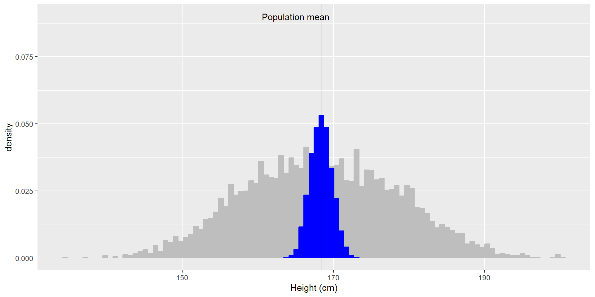
Let’s use the NHANES dataset again and let’s assume it is the entire population. We can calculate the mean (\(\mu = 168.35\)) and standard deviation (\(\sigma = 10.16\)) as the population parameters. If we repeatedly sample 50 individuals, we get this:

sampleMean	sampleSD
164.582	8.631756
168.102	10.388759
167.206	9.812454
170.006	11.372477
168.512	11.101804

The sample means and SDs are similar, but not exactly equal to the population parameters.

If we sample 5000 times (50 individuals each), we can see that the average of these 5000 sample means (depicted in blue) is similar to the population mean!
Average sample mean across 5000 sample: \(\hat{X} = 168.3463\).

grey = population histogram (raw data) blue = sample means of samples with N=50

What is similar between these distributions? What is different?

Standard Error of the Mean

In the example on the last slide, the means were all pretty close to each other, i.e. the blue distribution was very narrow and the variance small (compared to the grey distribution). This is an inherent statistical property of sample means: By averaging several individual values, thus aggregating them into a sample (here with \(n = 50\)), we reduce the variability of the sampling distribution.

We can quantify this variability of the sample mean with the standard error of the mean (SEM).

\[SEM = \frac{\hat{\sigma}}{\sqrt{n}}\]

This formula needs two values: the population variability \(\sigma\) (or sample SD \(\hat{\sigma}\) as approximation) and the size of our sample \(n\).

We can only control our sample size, thus if we want a better estimate, we can increase sample size!

A sample of \(n = 50\) already decreases the population variability by a factor of \(\sqrt{50} = 7.1\) !

SEM ~ SD of sampling distribution of the mean

Takes the SD of the data and divides it by sample size (so always smaller than SD!)

We use the sample SD as an approximation for the population SD

Use the sigma of the data? same as sd(sample_means)

“the utility of larger samples diminishes with the square root of the sample size”: Doubling the sample size will not double the quality of the statistic.

The Central Limit Theorem

The Central Limit Theorem (CLT) is a fundamental (and often misunderstood) concept of statistics.

CLT: With larger sample sizes, the sampling distribution of sample means (i.e., the blue distribution from before) will become more and more normally distributed*, even if the population distribution is not (i.e., the grey distribution from before)!

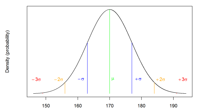
Normal Distribution of Height

Note: Means approximate a normal distribution, irrespective of the distribution from which the data stem. This is because the sampling error between the sampling mean \(\hat{\mu}\) and the population mean \(\mu\) follows a normal distribution.

Described by mean and sd: Shape never changes, only location and width!

CLT in Action

On the left you can see a highly skewed distribution of alcohol consumption per year (from the NHANES dataset). If we repeatedly draw samples of size 50 from the datset and take the mean, we get the right distribution of sample means - which looks a lot more “normal” (normal distribution is added in red)!

The CLT is important because it allows us to safely assume that the sampling distribution of the mean will be normal in most cases, which is a necessary prerequisite for many statistical techniques.

Red peak: True population mean Blue values left of peak: Sampling error with underestimation of the true population mean Blue values right of peak: Sampling error with overestimation of the true population mean

Resampling and Simulation

Simulations

As you saw in last lecture, we can also use similar functions (usually starting with r) to simulate data (i.e., to draw samples from probability distributions).

This can be helpful if we don’t know the “ground truth” or want to quantify uncertainty. We can also use simulations to calculate the power of a study.

With simulations, we define the expected “ground truth” (distribution of the population) and generate data from it.

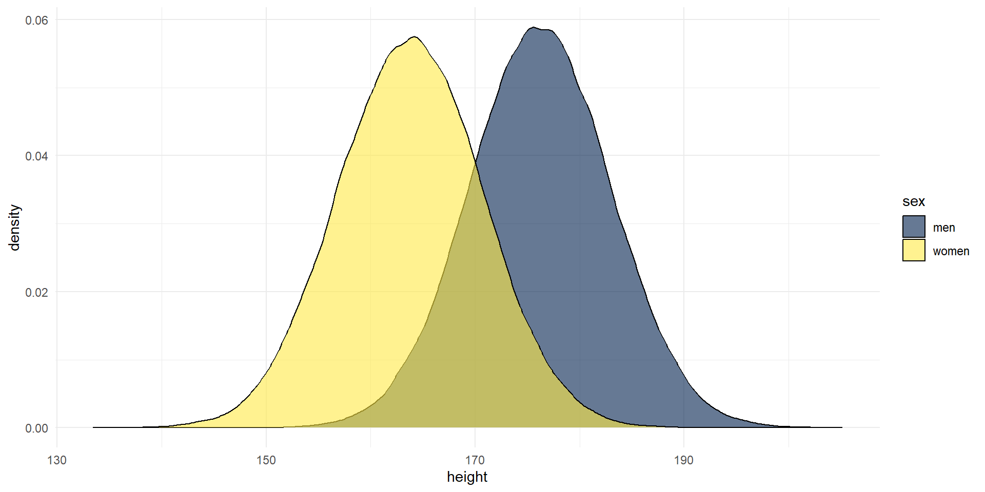
Example: We can use rnorm() to simulate data from a normal distribution with given parameters. Here, we will use means and SDs from the Scottish Health Survey (2008) to visualize two normal distributions:

men <- rnorm(n = 100000, mean = 176.2, sd = 6.748) 
women <- rnorm(n = 100000, mean = 163.8, sd = 6.931)  
heights <- tibble(men, women) %>%   
  pivot_longer(names_to = "sex", values_to = "height", men:women)  
heights %>% 
  ggplot(aes(x = height, fill = sex)) +   
  geom_density(alpha = .6) +   
  scale_fill_viridis_d(option = "E") +   
  theme_minimal()

We could use these data to visualize how much overlap there is between the two distributions of men and women, or to test how big the difference in height needs to be to become significant etc.

We use “real data” as input for the simulations! So the simulations are based on empirical values (means, sd), but we actually draw more observations, 100.000!

Simulate Different Distributions

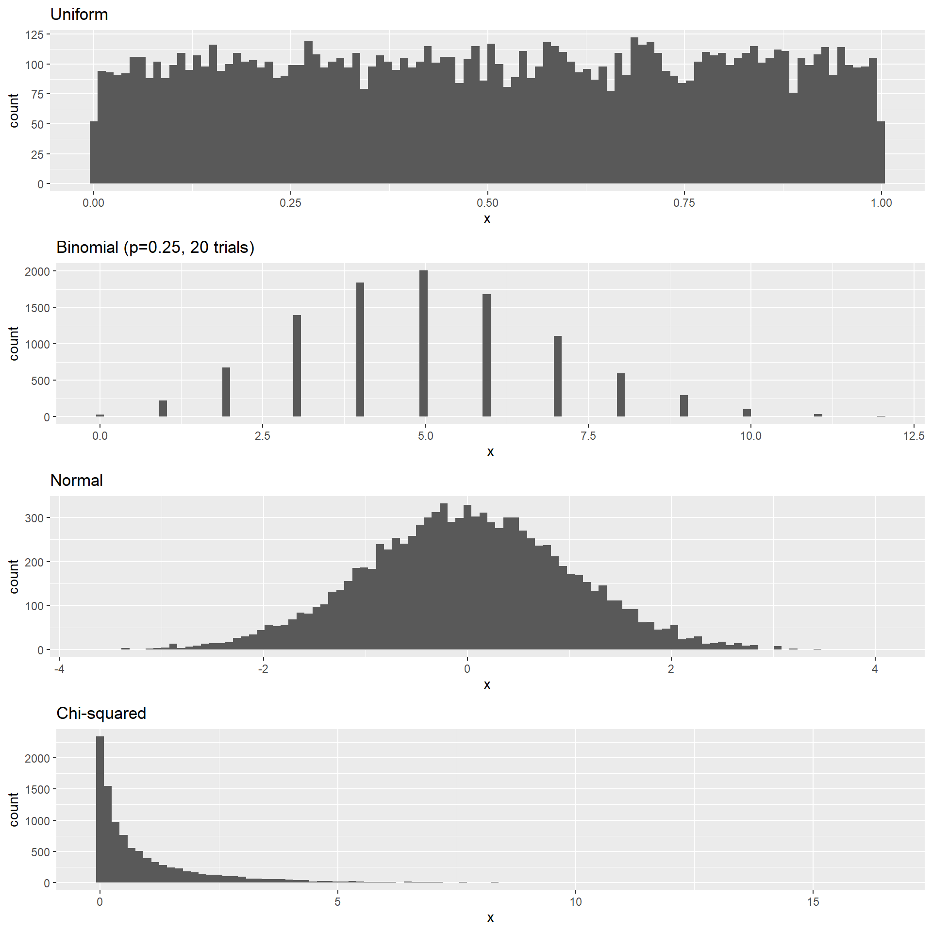
It is possible to draw data from different distributions:

nsamples <- 10000 
nhistbins <- 100  

# uniform distribution 
p1 <- tibble(x = runif(nsamples)) %>%    
  ggplot((aes(x))) + 
  geom_histogram(bins = nhistbins) +    
  labs(title = "Uniform")  

# binomial distribution 
p2 <- tibble(x = rbinom(nsamples, 20, 0.25)) %>%    
  ggplot(aes(x)) + 
  geom_histogram(bins = nhistbins) +   
  labs(title = "Binomial (p=0.25, 20 trials)")  

# normal distribution 
p3 <- tibble(x = rnorm(nsamples)) %>%    
  ggplot(aes(x)) + 
  geom_histogram(bins = nhistbins) +   
  labs(title = "Normal")  

# Chi-squared distribution 
p4 <- tibble(x = rchisq(nsamples, df=1)) %>%    
  ggplot(aes(x)) + 
  geom_histogram(bins = nhistbins) +   
  labs(title = "Chi-squared")  

cowplot::plot_grid(p1, p2, p3, p4, ncol = 1)

Simulate a Fake Dataset

Let’s simulate data of 120 participants of different heights and genders flipping a coin. To do so, we need to know how to simulate a) heights, b) flip a coin, and c) assign genders.

Simulate heights:

heights <- rnorm(120, mean = 170, sd = 10)

Simulate coin flips:

(Instead of drawing from a probability distribution function that starts with an r, e.g. rnorm(), we use sample(), which randomly (uniformly) draws from values you determine. We need to set replace=TRUE)

coin_flips <- sample(c("Head", "Tail"), 120, replace=TRUE) 

We could of course use similar code to simulate gender or the like.

But if we want to predetermine which genders we want to collect data from (i.e. same number in each gender group), we can also use the function rep(). This function will simply repeat an observation for a number of rows:

genders <- rep(x = c("man", "woman", "nonbinary"), each = 40) #%>% sample() 
#you can run just "sample" on a vector to randomize its order 

Determine participant numbers and combining everything into one dataframe:

sim_data <- tibble(   
  participant_number = 1:120,   
  gender = rep(x = c("man", "woman", "nonbinary"), each = 40),   
  height = rnorm(120, mean = 170, sd = 10),   
  coin_flip = sample(c("Head", "Tail"), 120, replace=TRUE) )  

# or if you have run all the code before, you could also use the objects you have already in your Environment: 
# sim_data <- tibble(participant_number = 1:120, genders, heights, coin_flips)

If we wanted to do a Monte Carlo Simulation, we could use the code from the last slide and put the simulation into a for loop. Inside the for loop, we would also calculate some value of interest (one estimate per subsample, such as the mean).

Monte Carlo Simulation

With the increasing use of computers, simulations have become an essential part of modern statistics. Monte Carlo simulations are the most common ones in statistics.

There are four steps to performing a Monte Carlo simulation:

1. Define a domain of possible values.

2. Generate random numbers within that domain from a probability distribution.

3. Perform a computation using the random numbers.

4. Combine the results across many repetitions.

Randomness in Statistics

Random = unpredictable.

For a Monte Carlo simulation, we need pseudo-random* numbers, which are generated by a computer algorithm.

We can simply generate (pseudo-)random numbers from different distributions with R, e.g. with rnorm() to draw (pseudo-)random numbers from a normal distribution:

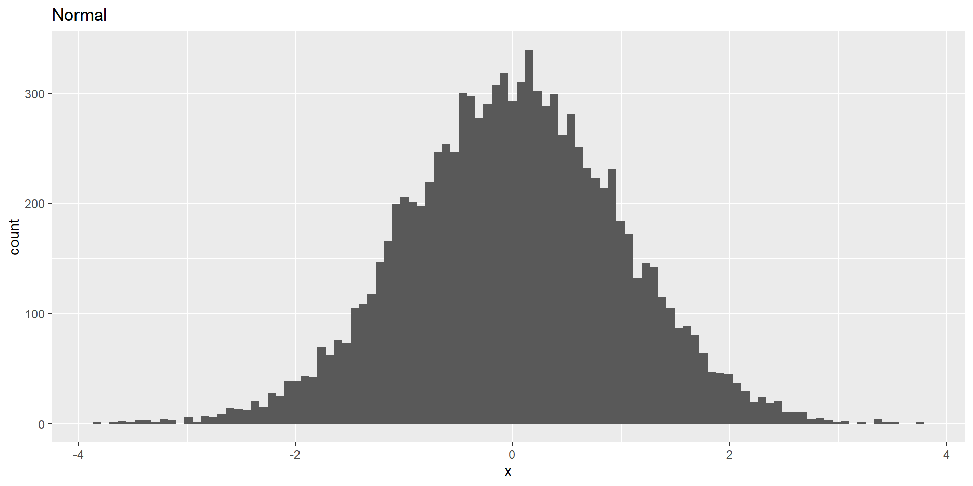
# Draw 10000 random numbers of a normal distribution with mean=0, sd=1
rand_num <- rnorm(n=10000, mean=0, sd=1)

# Plot the random numbers and verify that they make up a normal distribution
tibble(x = rand_num) %>% 
  ggplot(aes(x)) +
  geom_histogram(bins = 100) +
  labs(title = "Normal")

Each time, we generate random numbers, these will differ slightly.

But we can also generate the exact same set of random numbers (which will be helpful to reproduce results!) by setting the random seed to a specific value such as 123: set.seed(123).

rnorm(): Here, r stands for random normal distribution

Flip a coin, we don’t know the outcome! (Only if we knew a lot of physics and the conditions…)

Humans have a bad sense of randomness, we think we see patterns everywhere (gambler’s fallacy: being due for a win).

* Truly random numbers, that are completely unpredictable, are only possible through physical processes that are difficult to obtain.

Pseudo-random numbers will only seem random (they are difficult to predict) but will repeat at some point.

Using Monte Carlo Simulations

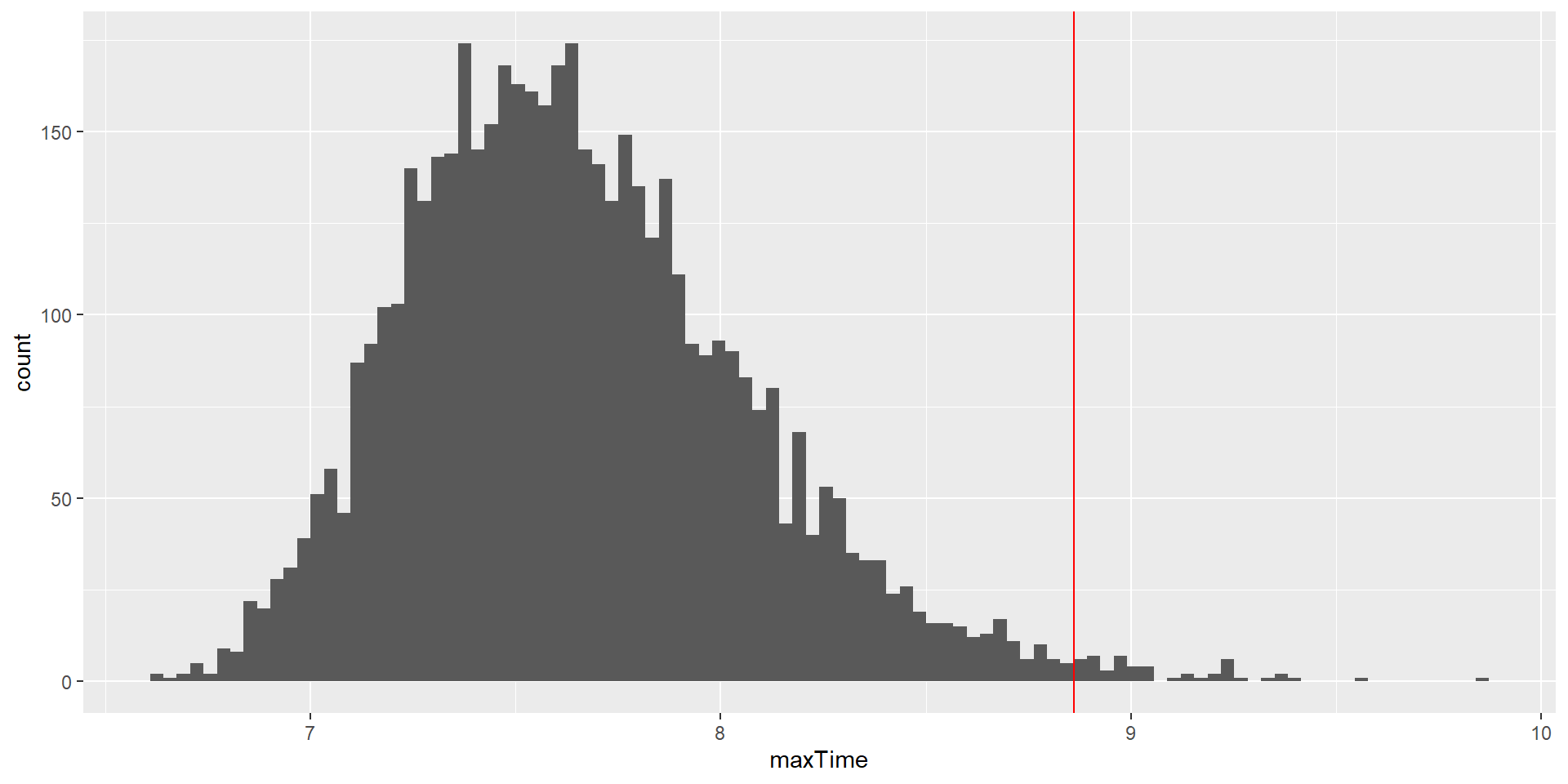
Example: Let’s try to find out how much time we should allow for a short in-class quiz.

We pretend to know the distribution of completion times is normal, with mean = 5 min and SD = 1 min.

How long does the test period need to be so that we can expect ALL students (n = 150) to finish in 99% of the quizzes?

To answer this question, we need the distribution of the longest finishing time.

What we will do is to simulate finishing times for a great number of quizzes and take the maximum of each (the longest finishing time). We can then look at the distribution of maximum finishing times and see where the 99% quantile is.
This value is the amount of time that we should allow - given our assumptions!!

Using Monte Carlo Simulations 2

Let’s repeat the steps of the simulation by going through the four steps mentioned before:

1. Define a domain of possible values.

–> Our assumptions: The values would come from a normal distribution with \(n = 150\), \(mean = 5\), and \(SD = 1\).

2. Generate random numbers within that domain from a probability distribution.

rand_num <- rnorm(n = 150, mean = 5, sd = 1)

3. Perform a computation using the random numbers.

max_rand_num <- max(rand_num) #time of slowest student

Using Monte Carlo Simulations 3

4. Combine the results across many repetitions.

nrep <- 5000 #number of repetitions

# initialize an empty matrix to fill in the max values later
max_rand_num <- matrix(data = NA, nrow = nrep, ncol=1)

# use a for-loop to repeat resampling nrep times!
for (i in 1:nrep) {
  rand_num <- rnorm(n = 150, mean = 5, sd = 1)
  max_rand_num[i, 1] <- max(rand_num)
}

# get the cutoff (99%) of the distribution of max values
cutoff <- quantile(max_rand_num, 0.99)
print(cutoff)

     99% 
8.793609 

Using Monte Carlo Simulations 4

This shows that the 99th percentile of the finishing time distribution falls at 8.8602684 minutes, meaning that if we were to give that much time for the quiz, then we expect that in 99% of quizzes, every student would finish.

Assumptions matter, otherwise results wrong! (We assumed: normal dist w/ particular mean and SD). Here assumptions certainly wrong –> elapsed time not normal

Resampling: The Bootstrap

We can use simulations to demonstrate statistical principles (like we just did) but also to answer statistical questions.

The bootstrap is a simulation technique that allows us to quantify our uncertainty of estimates!

1. We repeatedly sample with replacement from an actual dataset.
2. We compute a statistic of interest for each sample.
3. We get the distribution of those statistics and use it as our sampling distribution.

Bootstrap Example

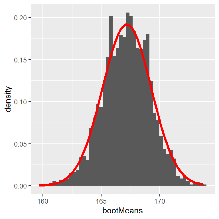
Let’s use the bootstrap to estimate the sampling distribution of the mean heights of the NHANES dataset. We can then compare the result to the SEM (=uncertainty of the mean) that we discussed earlier.

# perform the bootstrap to compute SEM and compare to parametric method
nRuns <- 2500
sampleSize <- 32

heightSample <- 
  NHANES_adult %>%
  sample_n(sampleSize) # draw 32 observations

# function to bootstrap (sample w/ replacement) & get mean
bootMeanHeight <- function(df) {
  bootSample <- sample_n(df, dim(df)[1], replace = TRUE)
  return(mean(bootSample$Height))
}

# run function 2500x
bootMeans <- replicate(nRuns, bootMeanHeight(heightSample))

# calculate "normal" SEM and bootstrap SEM
SEM_standard <- sd(heightSample$Height) / sqrt(sampleSize)
SEM_bootstrap <- sd(bootMeans)

SEM_standard

[1] 2.081422

SEM_bootstrap

[1] 2.008614

An example of bootstrapping to compute the standard error of the mean adult height in the NHANES dataset. The histogram shows the distribution of means across bootstrap samples, while the red line shows the normal distribution based on the sample mean and standard deviation.

Evaluation: Bootstrapping

Con
Takes very long to compute (compared to the SEM)
Precision depends on computing time

Pro
No assumption about sampling distribution necessary
Is a good solution if you do not want to rely on certain assumptions

Bootstrapping is a so-called model-free procedure: You put in just the data and get a result that does not depend on any further assumptions.
Model-based procedures (like most statistical tests we will cover in this class) are usually more precise if their assumptions are met. Unfortunately, assumptions are not always straightforward to check.

Resampling

Let’s look at the Bootstrap. Remember that we usually use real data for bootstrapping and draw samples with replacement of the same size as the original dataset. We can use this to quantify uncertainty, such as with the Standard Error of the Mean (SEM) or Confidence Intervals.

Let’s say we have a very small sample of “sweets consumed”. We don’t know the underlying distribution. We make up a dataset, but let’s pretend it is our real data:

data_10 <- tibble(
  participant = 1:10,
  sweets = c(5, 5, 5, 7, 3, 3, 4, 6, 8, 4)
)

We want to know how sample size influences the SEM, so we also have a sample with twice 10x as many observations:

data_20 <- tibble(
  participant = 1:100,
  sweets = rpois(100,4) #random Poisson distribution
)

Resampling 3

Let’s resample 1000 times. To get the sampling distributions of the means, we have to save each mean of each iteration:

set.seed(8465123)
iterations <- 1000 

# initialize empty matrices
mean_bootstrap_10 <- matrix(NA, nrow = iterations, ncol = 1)
mean_bootstrap_20 <- matrix(NA, nrow = iterations, ncol = 1)

for (i in 1:iterations) {
  # draw exactly the same amount of datapoints as in the original dataset, but with replacement
  bootstrap_data_10 <- sample_n(data_10, 10, replace=TRUE)
  bootstrap_data_20 <- sample_n(data_20, 20, replace=TRUE)
  
  # calculate the mean for each of the subsamples, put it into matrix in subsequent rows
  mean_bootstrap_10[i,1] <- mean(bootstrap_data_10$sweets)
  mean_bootstrap_20[i,1] <- mean(bootstrap_data_20$sweets)
}

# calculate the SEMs
sd(mean_bootstrap_10)

[1] 0.4948013

sd(mean_bootstrap_20)

[1] 0.4638429

We can conclude that the SEM is smaller with a larger sample size, which means we can be more certain about our estimate! (We already knew this from the \(\sqrt{n}\) in the denominator of the SE formular but it’s nice to see it confirmed.)

Thanks!

Learning objectives:

• Understand why we are sampling from a population and what the sampling distribution (and the sampling error) is.

• Understand Monte Carlo Simulations and the Bootstrap, and being able to implement those in R.

Next:

Hypothesis testing! Finally! :D