08 Modeling Relationships

Julius-Maximilians-University Würzburg
Course: “Biostatistics”
Translational Neuroscience

Dr. Mario Reutter (slides adapted from Dr. Lea Hildebrandt)

Agenda

• Categorical Relationships (Chi² tests)
• Continuous Relationships (Correlations)
• Group Comparisons (t-tests & ANOVA)

Modeling Categorical Relationships

Now that we have covered the basics, we will apply them and turn to the question how to model particular relationships.

Chi² Test: General

We will first focus on modeling categorical relationships (i.e., of variables that are qualitative!).

These data are usually expressed in terms of counts.

Example: Candy colors

Bag of candy: 30 chocolates, 33 licorices, and 37 gumballs.

Is the distribution fair (i.e., 1/3rd of the bag for each candy) and the fact that there are only 30 chocolates within expectations?

What is the likelihood that the count would come out this way (or even more extreme) if the true probability of each candy type is the same?

Counts: For each combination of variables, how many observations do we have?

If the machine really sorts on average 1/3 of each in each bag? How much is due to chance?

Chi² Test: One Variable

The Chi² test checks whether observed counts differ from expected values (\(H_0\)).

\[ \chi^2 = \sum_i\frac{(observed_i - expected_i)^2}{expected_i} \]

The null hypothesis in our example is that the proportion of each type of candy is equal (1/3 or ~33.33).

If we plug in our values from above, we would calculate \(\chi^2\) like this:

\[ \chi^2 = \frac{(30 - 33.33)^2}{33.33} + \frac{(33 - 33.33)^2}{33.33} + \frac{(37 - 33.33)^2}{33.33} = 0.74 \]

take the difference between observed and expected (33.33), square it, divide it by expected 33.33 and add everything up

Chi² Test: General

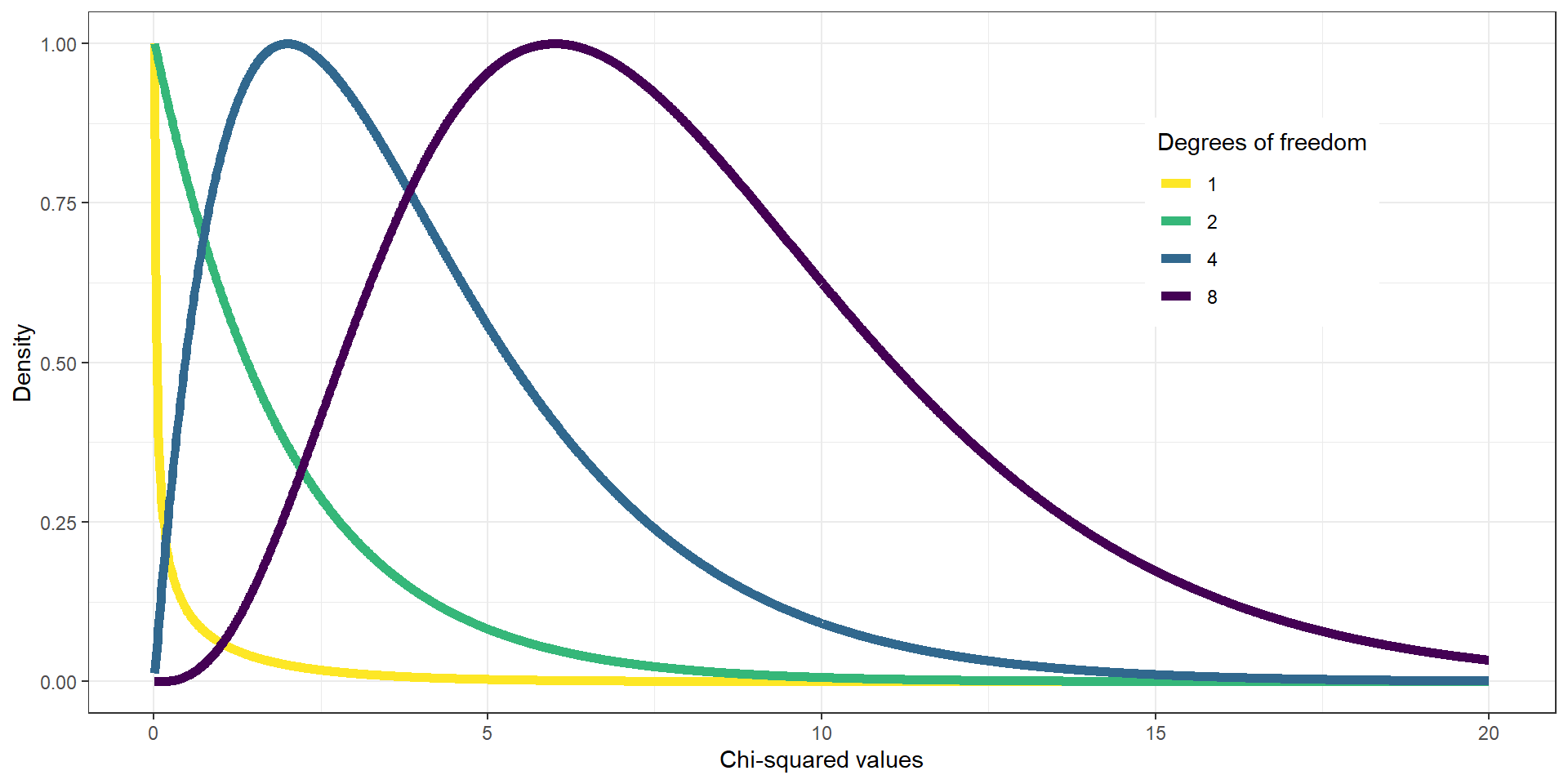
On its own, the \(\chi^2\) statistic is not interpretable - it depends on its distribution.

The shape of the \(\chi^2\) distribution depends on the degrees of freedom (much like the t distribution), which is the number of category levels \(k-1\).

Chi2 Test: Candies

For the candy example, we use a chi-squared distribution with \(DFs = 2\) (3 candy categories minus one → green line). If we’d look at the distribution and found \(\chi^2 = .74\) on the x-axis (dashed red line), we would see that it does not fall far into the tail of the distribution but is rather in the middle. If we calculate the p-value, we’d get \(P(\chi^2 > .74) = 0.691\).

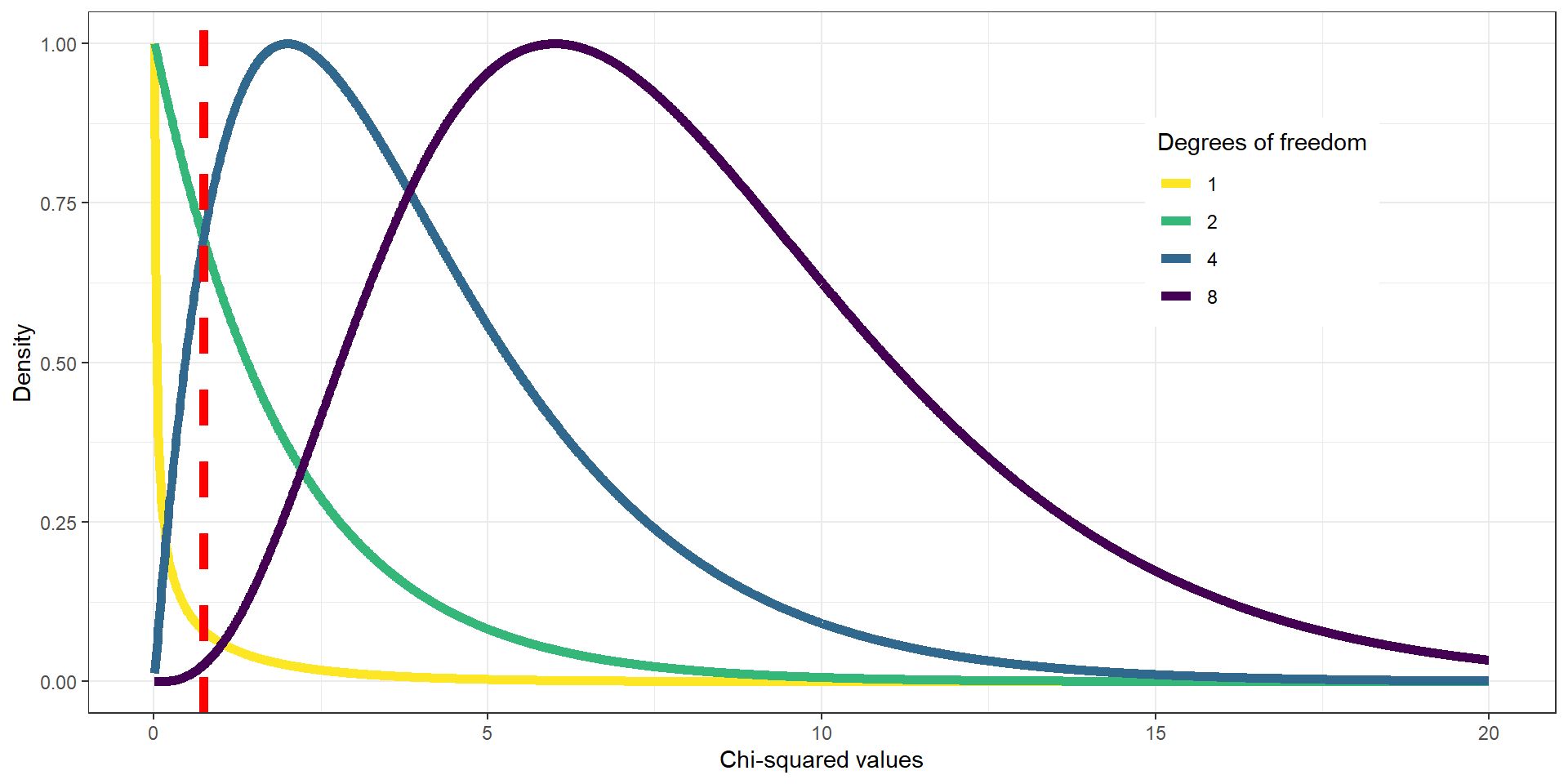
It is thus not particularly surprising to find this distribution of candies and we would not reject \(H_0\) (equal proportions).

Contingency Tables and the Two-Way Test

The \(\chi^2\) test is also used to test whether two categorical variables are related to each other.

Example: Are Black drivers more likely to be pulled over by police than white drivers?

We have two variables: Skin color (black vs white) and being pulled over (true vs. false). We can represent the data in a contingency table (remember: the count() function was helpful to do this in R):

Contingency table for police search data

searched	Black	White	Black (relative)	White (relative)
FALSE	36244	239241	0.1295298	0.8550062
TRUE	1219	3108	0.0043565	0.0111075

Contingency Tables and the Two-Way Test

If there is no relationship between skin color and being searched, the frequencies of searches would be proportional to the frequencies of skin color. This would be our expected values. We can determine them using probabilities:

	Black	White
Not searched	\(P(\neg S)*P(B)\)	\(P(\neg S)*P(W)\)	\(P(\neg S)\)
Searched	\(P(S)*P(B)\)	\(P(S)*P(W)\)	\(P(S)\)
	\(P(B)\)	\(P(W)\)	\(100\%\)

Remember: You can only multiply two probabilities to get their conjoint probability if they are independent. Here, we assume independence to calculate expected values and then check how much our observed values deviate from independence.

Probabilities: Because we expect the variables to be unrelated, we can calculate the joint probability as the product of the marginal probabilities:
\(P(X \cap Y) = P(X) * P(Y)\)

Marginal probabilities are the prob of each event occuring regardless of other events (in the margins of the table!)

Chi² Test with Two Variables

If we compute the standardized squared difference between observed and expected values, we can sum them up to get \(\chi^2 = 828.3\)

Contingency table for police search data

searched	driver_race	n	expected	stdSqDiff
FALSE	Black	36244	36883.67	11.09
TRUE	Black	1219	579.33	706.31
FALSE	White	239241	238601.33	1.71
TRUE	White	3108	3747.67	109.18

We can then compute the p-value using a chi-squared distribution with \(DF = (levels_{var1} - 1) * (levels_{var2} - 1) = (2-1) * (2-1) = 1\)

Chi² Test with Two Variables in R

We can calculate a \(\chi^2\) test easily in R:

chisq.test(summaryDf2wayTable, correct = FALSE)

    Pearson's Chi-squared test

data:  summaryDf2wayTable
X-squared = 828.3, df = 1, p-value < 2.2e-16

The results indicate that the data are highly unlikely if there was no true relationship between skin color and police searches! We would thus reject \(H_0\).

DF: computing the expected frequencies requires three values: total number of observations and marg probs each variable. thus only one of the four values can vary freely.

Chi² Test with Two Variables: Interpretation

Question: What is the direction of the observed relationship?

Contingency table for police search data

searched	driver_race	n	expected	stdSqDiff
FALSE	Black	36244	36883.67	11.09
TRUE	Black	1219	579.33	706.31
FALSE	White	239241	238601.33	1.71
TRUE	White	3108	3747.67	109.18

Standardized Residuals

If we want to know not only whether but also how the data differ from what we would expect under \(H_0\), we can examine the residuals of the model.

The residuals tell us for each cell how much the observed data deviates from the expected data.

To make the residuals better comparable, we will look at the standardized residuals:

\[ \text{standardized residual}_{ij} = \frac{observed_{ij} - expected_{ij}}{\sqrt{expected_{ij}}} \]

where \(i\) and \(j\) are the rows and columns respectively.

Standardized Residuals

Negative residuals indicate an observed value smaller than expected.

Summary of standardized residuals for police stop data

searched	driver_race	Standardized residuals
FALSE	Black	-3.330746
TRUE	Black	26.576456
FALSE	White	1.309550
TRUE	White	-10.449072

raw residuals depend on number of observations!

Black individuals are searched way more often than expected –> helps us intepret significant results.

Odds Ratios

Alternatively, we can represent the relative likelihood of different outcomes as odds ratios:

\[ odds_{searched|black} = \frac{N(searched\cap black)}{N(\neg searched \cap black)} = \frac{1219}{36244} = 0.034 \]

\[ odds_{searched|white} = \frac{N(searched \cap white)}{N(\neg searched \cap white)} = \frac{3108}{239241} = 0.013 \]

\[ odds\ ratio = \frac{odds(searched|black)}{odds(searched|white)} = 2.59 \]

The odds of being searched are 2.59x higher for Black vs. white drivers!

Simpson’s Paradox

The Simpson’s Paradox is a great example of misleading summaries.

If we look at the baseball data below, we see that David Justice has a better batting average in every single year, but Derek Jeter has a better overall batting average:

Player	1995		1996		1997		Combined
Jeter	12/48	.250	183/582	.314	190/654	.291	385/1284	.300
Justice	104/411	.253	45/140	.321	163/495	.329	312/1046	.298

How can this be?

Simpson’s Paradox: A pattern is present in the combined dataset but may be different in subsets of the data.

Happens if another (lurking) variable changes across subsets (e.g., the number of at-bats, i.e., the denominator).

batting average: hits/at bats

1995: in general low batting averages, Justice had a lot of at-bats => diminishes total combined value more strongly than for Jeter.

1996: both players were above their average but Jeter had way more at-bats => more important for the overall average.

Simpson’s Paradox: More intuitive

While typing on a keyboard, what is the relationship between speed (words per minute) and accuracy (% correct words)? (positive, negative, or none)

If I try to type faster, I will make more errors ⇒ speed-accuracy trade-off (negative association)

People who are better at typing usually are both faster and make fewer mistakes (positive association)

Answer: It depends

• Within a person, the relationship between speed and accuracy is negative. My own skill is limited, I can either use it for speed or accuracy.
• Between persons, the relationship is positive due to inter-individual differences in overall typing skill.

Usually, when leveling up, people don’t put all their skill points in only speed or accuracy.

Modeling Continuous Relationships

Example: Income Inequality and Hate Crimes

We want to look at a dataset that was used for an analysis of the relationship between income inequality (Gini index) and the prevalence of hate crimes in the USA.

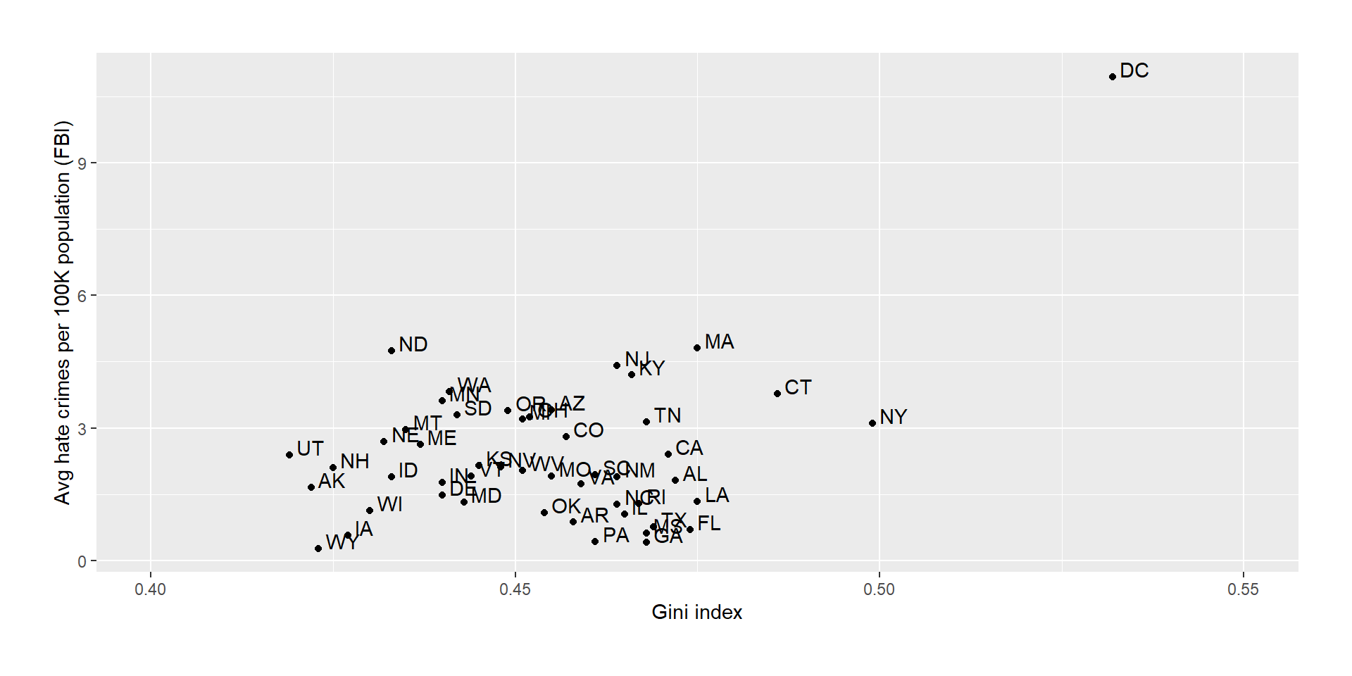
It looks like there is a positive relationship between the variables. How can we quantify this relationship?

Covariance and Correlation

Variance (single variable): \(s^2 = \frac{\sum_{i=1}^n (x_i - \bar{x})^2}{N - 1}\)

Covariance (two variables): \(covariance = \frac{\sum_{i=1}^n (x_i - \bar{x})(y_i - \bar{y})}{N - 1}\)

“Is there a relation between the deviations of two different variables (from their means) across observations?”

Covariance will be far from 0 if data points share a relationship. Positive values for same direction, negative values for opposite directions.

Covariance varies with overall level of variance in the data ⇒ hard to compare different relationships

Correlation coefficient (Pearson correlation): Scales the covariance by the standard deviations of the two variables and thus standardizes it (→ \(r\) varies between \(-1\) and \(1\) ⇒ comparability!)

\[ r = \frac{covariance}{s_xs_y} = \frac{\sum_{i=1}^n (x_i - \bar{x})(y_i - \bar{y})}{(N - 1)s_x s_y} \]

Insight: Variance is the covariance of a variable with itself.

Covariance depends on dataset and even on scaling of variables!
e.g. relationship between body height and weight ⇒ Using m vs. cm for height will change variance and thus covariance even though the relationship should be identical (same data)

Hypothesis Testing for Correlations

The correlation between income inequality and hate crimes is \(r = .42\), which seems to be a reasonably strong (positive) relationship.

We can test whether such a relationship could occur by chance, even if there is actually no relationship. In this case, our null hypothesis is \(H_0: r = 0\).

To test whether there is a significant relationship, we can transform the \(r\) statistic into a \(t\) statistic:

\[ t_r = \frac{r\sqrt{N-2}}{\sqrt{1-r^2}} \]

Correlation in R

# perform correlation test on hate crime data
cor.test(
  hateCrimes$avg_hatecrimes_per_100k_fbi,
  hateCrimes$gini_index
)

    Pearson's product-moment correlation

data:  hateCrimes$avg_hatecrimes_per_100k_fbi and hateCrimes$gini_index
t = 3.2182, df = 48, p-value = 0.002314
alternative hypothesis: true correlation is not equal to 0
95 percent confidence interval:
 0.1619097 0.6261922
sample estimates:
      cor 
0.4212719 

The p-value is quite small, which indicates that it is quite unlikely to find an \(r\) value this high or more extreme with 48 degress of freedom. We would thus reject \(H_0: r = 0\).

subsetting with $!

Side note: There are more beautiful & convenient ways to do this in R. We will cover this in the next session.

Robust Correlations

In the plot, we have seen an outlier: The District of Columbia was quite different from the other data points.

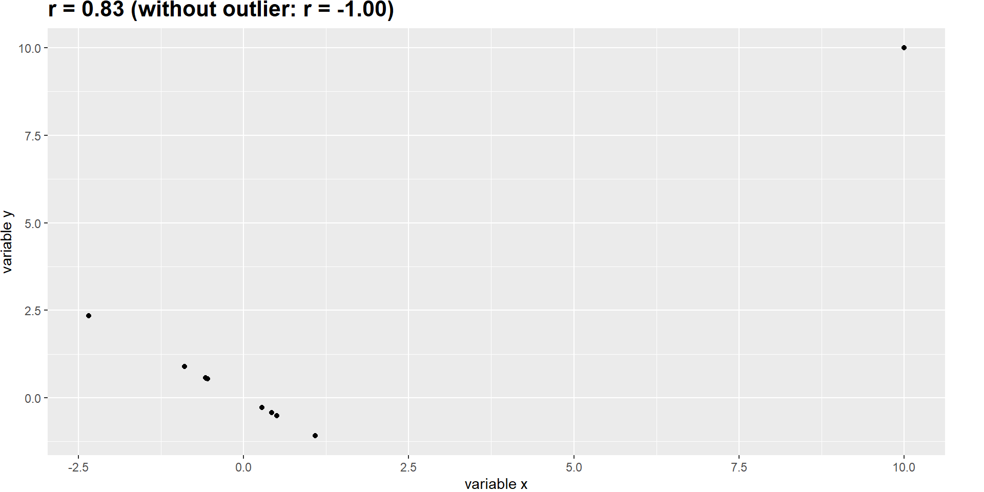
The Pearson’s correlation coefficient \(r\) is highly sensitive to outliers, see this hypothetical example:

Robust Correlation 2

We can use a different correlation coefficient, which is less sensitive to outliers: Spearman correlation.

It is based on ranking (i.e., ordering) the data and using the ranks (instead of the original data) for the correlation.

cor.test(hateCrimes$avg_hatecrimes_per_100k_fbi,
  hateCrimes$gini_index,
  method = "spearman")

    Spearman's rank correlation rho

data:  hateCrimes$avg_hatecrimes_per_100k_fbi and hateCrimes$gini_index
S = 20146, p-value = 0.8221
alternative hypothesis: true rho is not equal to 0
sample estimates:
       rho 
0.03261836 

The correlation has now dropped from \(.42\) to \(.03\) and is no longer significant.

Of course, a ranked correlation can also obscure true effects that critically depend on the scale of the data. When in doubt, try both and discuss reasons for differences.

Without outlier: perfectly negative correlation, with outlier: highly positive!

Correlation and Causation

Doing a well controlled, randomized experiment (RCT) is extremely helpful to gather causal evidence. However, it is not always possible or ethical to do an experiment!

Without an experiment, we can still collect observational data. However, if we correlate two observed variables, we can’t conclude that one causes the other: They (likely) share a relationship but there could also be a third variable that causes both (or even more complex causal structures).

Causal Graphs

If we have observational data, causal graphs can be helpful for interpreting causality:

Circle: observed variables
rectangle: latent (unobservable) variable

Green arrow: positive relationship,
red: negative

ExamGrade and FinishTime seem negatively related if we ignore other variables!
(“Hand in your exam early to improve your grade!”)

Knowledge = theoretical mediator
StudyTime = proxy for knowledge

If we control for StudyTime (which approximates individual knowledge), we find out that ExamGrade and FinishTime are (causally) unrelated!

We have briefly talked about causation in week 1

Think of data/questions where it is impossible/unethical!
abused children and brain development!
(3rd var: family stress -> less intellectual engagement –> poorer brain dev)

Correlation: s.th. is probably causing s.th. else but not clear what causes what!

DAG:
green: pos, red: net
circle: observed, rect: latent (unobservable)
ExamGrade and FinishTime seem neg related if we ignore others
knowledge = mediates
StudyTime = proxy for knowledge, if we “control” it/hold it constant/only use people with same amount, we would see that EG and FT are unrelated!

Comparing Means (Group Differences)

Testing a Single Mean (One sample t-Test)

We sometimes might want to know whether a single value, the mean of a group, differs from a specific value, e.g. whether the blood pressure in the sample differs from or is bigger than 80.

We can test this using the \(t\)-test, which we have already encountered in the “Hypothesis Testing” session!

\[ t = \frac{\hat{X} - \mu}{SEM} \]

\[ SEM = \frac{\hat{\sigma}}{\sqrt{n}} \]

\(\hat{X}\) is the mean of our sample, \(\mu\) the hypothesized population mean (e.g. the value we want to test against, such as 80 for the blood pressure example).

One sample t-Test in R

t.test(x=NHANES_adult$BPDiaAve, mu=80, alternative='greater')

    One Sample t-test

data:  NHANES_adult$BPDiaAve
t = -55.23, df = 4599, p-value = 1
alternative hypothesis: true mean is greater than 80
95 percent confidence interval:
 69.1588     Inf
sample estimates:
mean of x 
 69.47239 

The observed mean is actually much below 80, providing no evidence for our directional alternative hypothesis that it would be greater than 80 ⇒ the p values is (rounded to) 1.

If we had tested two-sidedly, we would have found a significant result. It may seem tempting now to create a story around an altered, non-directional alternative hypothesis, which is why it is important to preregister your hypotheses and analyses.

(The \(t\) statistic thus asks how large the deviation of sample mean from the expected value with respect to the sampling variability of the mean!)

We tested the one-sided alternative (>) and the blood pressure in the sample is much lower than 80, so it is far from significance

We can’t interpret the \(p\)-value as evidence in favor of \(H_0\) (i.e. larger \(p\)-value! vs non.sign) –> Bayes!

Comparing Two Means (Independent samples t-Test)

More often, we want to know whether there is a difference between the means of two groups.

Example: Do regular marijuana smokers watch more television?

\(H_0\) = marijuana smokers watch less or equally often TV,
\(H_A\) = marijuana smokers watch more TV.

If the observations are independent (i.e. you really have two unrelated groups), you can use a very similar formula to calculate the \(t\) statistic:

\[ t = \frac{\bar{X_1} - \bar{X_2}}{\sqrt{\frac{S_1^2}{n_1} + \frac{S_2^2}{n_2}}} \]

whereby \(\hat{X_1}\) and \(\hat{X_2}\) are the group means, \(S_1^2\) and \(S_2^2\) the group variances, and \(n_1\) and \(n_2\) the group sizes.

Independent samples t-Test in R

# t.test(NHANES_sample$TVHrsNum[NHANES_sample$RegularMarij=="Yes"],
#        NHANES_sample$TVHrsNum[NHANES_sample$RegularMarij=="No"],
#        alternative = "greater")

with(NHANES_sample, #only refer to data once using "with" function
     t.test(TVHrsNum[RegularMarij=="Yes"],
            TVHrsNum[RegularMarij=="No"],
            alternative = "greater"))

    Welch Two Sample t-test

data:  TVHrsNum[RegularMarij == "Yes"] and TVHrsNum[RegularMarij == "No"]
t = 1.2147, df = 116.9, p-value = 0.1135
alternative hypothesis: true difference in means is greater than 0
95 percent confidence interval:
 -0.09866006         Inf
sample estimates:
mean of x mean of y 
  2.30000   2.02963 

DV: continuous, IV: categories

n.s. (differs from book), although mean is higher in Yes, not significantly different!

Comparing Dependent Observations (Paired samples t-test)

If we have repeated observations of the same subject (i.e., a within-subject design), we might want to compare the same subject thus on multiple, repeated measurements.

If we want to test whether blood pressure differs between the first and second measurement session across individuals, we can use a paired \(t\)-test.

Side note: A paired \(t\)-test is equivalent to a one-sample \(t\)-test, when using the paired differences (\(X_2 - X_1\)) as \(\hat{X}\) and testing them against a value of 0 (if we expect no difference for \(H_0\)) for \(\mu\).

important: If we run an independent sample t-test, it would probably be n.s.! (check out book)

Paired samples t-test in R

t.test(NHANES_sample$BPSys1, NHANES_sample$BPSys2, paired = TRUE)

    Paired t-test

data:  NHANES_sample$BPSys1 and NHANES_sample$BPSys2
t = 2.7369, df = 199, p-value = 0.006763
alternative hypothesis: true mean difference is not equal to 0
95 percent confidence interval:
 0.2850857 1.7549143
sample estimates:
mean difference 
           1.02 

Comparing More Than Two Means

Often, we want to compare more than two means, e.g. different treatment groups or time points.

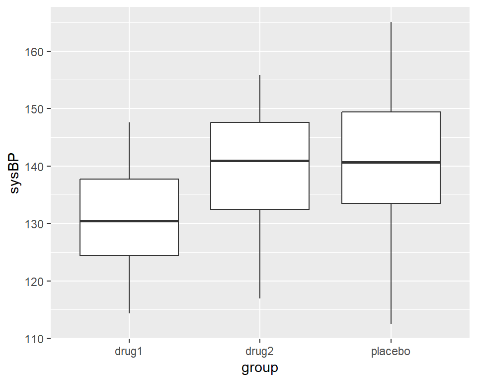
Example: Different treatments for blood pressure

Analysis of Variance (ANOVA)

\(H_0\): all means are equal
\(H_A\): not all means are equal (e.g. at least one differs)

We can partition the variance of the data into different parts:

\(SS_{total}\) = total variance in the data
\(SS_{model}\) = Variance explained by the model
\(SS_{error}\) = Variance not explained by the model

We can use those to calculate the mean squares for the model and the error:

\(MS_{model} =\frac{SS_{model}}{df_{model}}= \frac{SS_{model}}{p-1}\) (\(p\) is the number of factor levels or groups)

\(MS_{error} = \frac{SS_{error}}{df_{error}} = \frac{SS_{error}}{N - p}\) (\(N\) is the total sample size across groups)

quite common analysis! We will just scratch the surface

\(SS\) = Sum of Squares, remember that the variance is the sum of the squared deviation of an observation to the mean

\(MS\) = Mean (Sum of) Squares: How much variance per degree of freedom?

ANOVA in R

In R, we would run an ANOVA like this:

df <-
  df %>% 
  mutate(group2=fct_relevel(group,c("placebo","drug1","drug2")))
# reorder the factor levels so that "placebo" is the control condition/intercept!
  
 
# test model without separate duymmies
lmResultAnovaBasic <- lm(sysBP ~ group2, data=df)
anova(lmResultAnovaBasic)

Analysis of Variance Table

Response: sysBP
           Df  Sum Sq Mean Sq F value   Pr(>F)    
group2      2  2115.6 1057.81  10.714 5.83e-05 ***
Residuals 105 10366.7   98.73                     
---
Signif. codes:  0 '***' 0.001 '**' 0.01 '*' 0.05 '.' 0.1 ' ' 1

The \(F\)-statistic (also called omnibus test) actually tests our overall hypothesis of no difference between conditions.

ANOVA in R

We now know that not all groups should be considered equal. But where is the difference?

summary(lmResultAnovaBasic)

Call:
lm(formula = sysBP ~ group2, data = df)

Residuals:
     Min       1Q   Median       3Q      Max 
-29.0838  -7.7452  -0.0978   7.6872  23.4313 

Coefficients:
            Estimate Std. Error t value Pr(>|t|)    
(Intercept)  141.595      1.656  85.502  < 2e-16 ***
group2drug1  -10.237      2.342  -4.371 2.92e-05 ***
group2drug2   -2.027      2.342  -0.865    0.389    
---
Signif. codes:  0 '***' 0.001 '**' 0.01 '*' 0.05 '.' 0.1 ' ' 1

Residual standard error: 9.936 on 105 degrees of freedom
Multiple R-squared:  0.1695,    Adjusted R-squared:  0.1537 
F-statistic: 10.71 on 2 and 105 DF,  p-value: 5.83e-05

# emmeans(lmResultAnovaBasic, "group2" ) #run this to get means and CIs for each group

We can see a \(t\)-test for every drug against the placebo (remember we used fct_relevel for this). The \(t\)-tests show that drug1 (but not drug2) differs significantly from placebo.

ANOVA in R: Comments

In this simple example, we could have skipped the omnibus test (anova()) and just looked at the summary().

In practise, you will often run ANOVAs with several factors (grouping variables) that all have a multitude of factor levels (subgroups).
Think: Two groups of drugs and one placebo across four time points (before, during, after, & follow-up). This quickly creates too many possible comparisons to keep track of.

This complicates things furhter because then you can also have interactions between variables (e.g., drug1 does not work better but faster than drug2).

For these examples, it is helpful to first get an overall statement if a factor (or an interaction of factors) has an influence on the results. If this is the case, you can run the individual t-tests for this factor to get a more detailed look.

Thanks!

Learning objectives:

• What are contingency tables and how do we use \(\chi^2\)-tests to assess a significant relationship between categorical variables?

• Be able to describe what a correlation coefficient is as well as compute and interpret it.

• Know what a \(t\)-test & ANOVA is and how to compute and interpret them.

Next:

Practical exercises in R!