Dr. Mario Reutter & Juli Nagel
(slides adapted from Dr. Lea Hildebrandt)
R!
General: Working with R in this course
You should have RStudio open and your precision workshop project loaded (we will set up the project today).
Have the slides open in the background - handy to copy R code (top right button if you hover over a code chunk) or click on links.
If possible, use two screens with the slides (Zoom) opened on one and RStudio on the other
print("Hello World")
[1] "Hello World"
Note: You can navigate through the slides quickly by clicking on the three dashes in the bottom left.
Why write code?
Doing statistical calculation by hand? Tedious & error prone! Computer is faster…
Using spreadsheets? Limited options, change data accidentally…
Using point-and-click software (e.g., SPSS)?
proprietary software = expensive
R = open, extensible (community)
reproducible!
Science/Academia is a marathon and not a sprint
=> it is worthwhile investing in skills with a slow learning curve that will pay off in the long run
Why write code?
Managing Expectations
You will learn a new (programming) language. Don’t expect to “speak” it fluently right away.
During the workshop, it is more important that you can roughly comprehend written code and “translate” it into natural language.
The second step is to be able to make small adjustments to code that is given to you.
Only then, the last step is to be able to produce code yourself (with the help of Google, Stackoverflow, templates of this course, etc. :) ).
But: Use it or loose it! Don’t wait to use R in your research projects until you’re “good enough”. It’s more fun to use it on “actual” problems, and makes it much easier to learn.
Install R & RStudio
You should all have installed R & RStudio by now! Who had problems doing so?
Overview RStudio
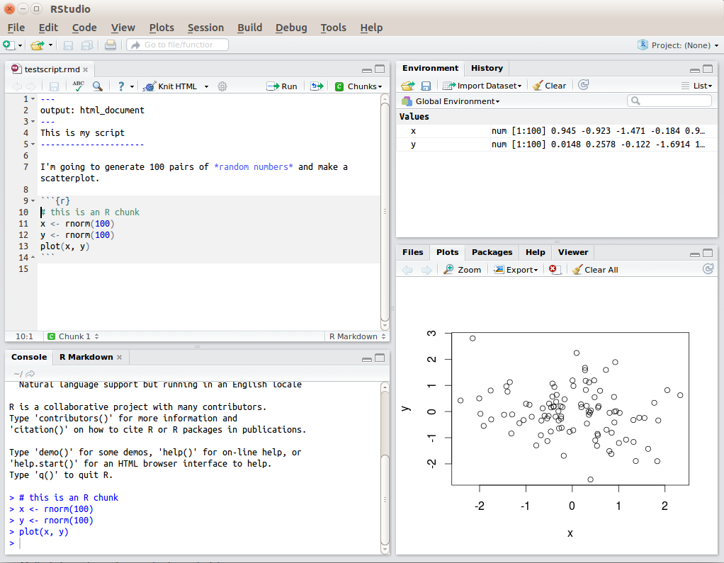
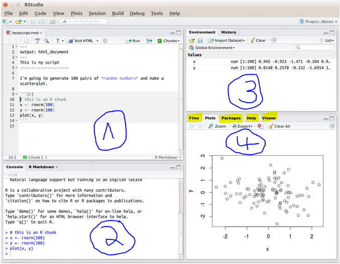
RStudio Interface
RStudio Panes
Script pane: view, edit, & save your code
Console: here the commands are run and rudimentary output may be provided
Environment: which variables/data are available
Files, plots, help etc.
RStudio Interface
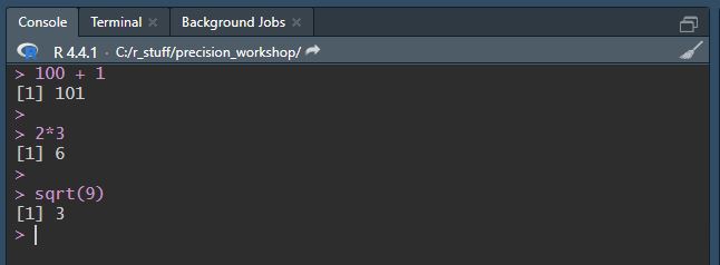
Using the Console as a Calculator
100+1
[1] 101
2*3
[1] 6
sqrt(9)
[1] 3
Console used as calculator
Saving the Results as a Variable/Object
a <-100+1multi <-2*3SqrtOfNine <-sqrt(9)word <-"Hello"
<- is used to assign values to variables (= is also possible, but discouraged in R)
a, multi etc. are the variable names (some naming rules, e.g., no whitespace, must not start with an number, many special characters not allowed)
You can find those now in your Environment! (top right panel)
No feedback in the console for saving variables (2*3 outputs 6, but multi <- 2*3 doesn’t)
variables can contain basically anything (words, numbers, entire tables of data …)
the variables contain the calculated value (i.e. 101) and not the calculation/formula (100+1)
Working with variables
a + multi
[1] 107
a
[1] 101
multi
[1] 6
You can use those variables for further calculations, e.g., a + multi
Note that neither a nor multi change their value.
Working with variables
a
[1] 101
a <-42a
[1] 42
Variables can be overwritten (R won’t warn you about this!)
Functions
This code with sqrt(9) looked unfamiliar. sqrt() is an R function that calculates the square root of a number. 9 is the argument that we hand over to the function.
If you want to know what a function does, which arguments it takes, or which output it generates, you can type into the console: ?functionname
?sqrt
This will open the help file in the Help Pane on the lower right of RStudio.
You can also click on a function in the script or console pane and press the F1 key.
Sometimes, the help page can be a bit overwhelming (lots of technical details etc.). It might help you to scroll down to the examples at the bottom to see the function in action!
Functions
Functions often take more than one argument (which have names):
rnorm(n =6, mean =3, sd =1)rnorm(6, 3, 1) # this outputs the same as above
You can explicitly name your arguments (check the help file for the argument names!) or just state the values (but these have to be in the correct order then! See help file).
rnorm(n =6, mean =3, sd =1)rnorm(6, 3, 1) # this outputs the same as abovernorm(sd =1, n =6, mean =3) # still the same resultrnorm(1, 6, 3) # different result - R thinks n = 1 and mean = 6!
Comments
rnorm(n =6, mean =3, sd =1)rnorm(6, 3, 1) # this outputs the same as above# By the way, # denotes a comment - very important for documentation!# Anything after # will be ignored by R# To (un)comment the line you are in/multiple lines you selected: ctrl + shift + C
Packages
There are a number of functions already included with Base R (i.e., R after a new installation), but you can greatly extend the power of R by loading packages (and we will!). Packages can e.g. contain collections of functions someone else wrote, or even data.
You should already have the tidyverse installed (if not, quickly run install.packages("tidyverse") :-) )
But installing is not enough to be able to actually use the functions from that package directly. Usually, you also want to load the package with the library() function. This is the first thing you do at the top of an R script:
library("tidyverse") # or library(tidyverse)
(If you don’t load a package, you have to call functions explicitly by packagename::function)
Scripts & Projects
If you type your code into the console (bottom left), it is not saved. Therefore, it is better practice to write scripts (top left) and save them as files.
Scripts are basically text files that contain your code and can be run as needed.
It makes sense to save all your scripts etc. in a folder specifically dedicated to this course.
We will now create an Rproject together, which will help you to work with files that belong together.
New Project
Create a new project by clicking on “File” on the top left and then “New Project…”
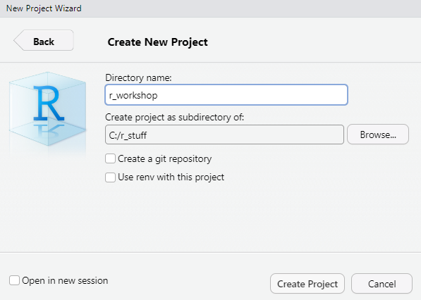
Select “New Directory” (if you already have a folder for this course, you can choose “Existing directory” and select that folder) and then choose “New Project” at the top of the list.
Choose a project name, e.g., as “r_workshop” (this will create a folder in which the project lives)
Browse where you want to put your project folder (in my case, “C:/r_stuff/”)
PS: R can deal with folder and file names that contain spaces, but since some programms can’t, it’s best practice not to use whitespaces for file/folder naming.
Existing Projects
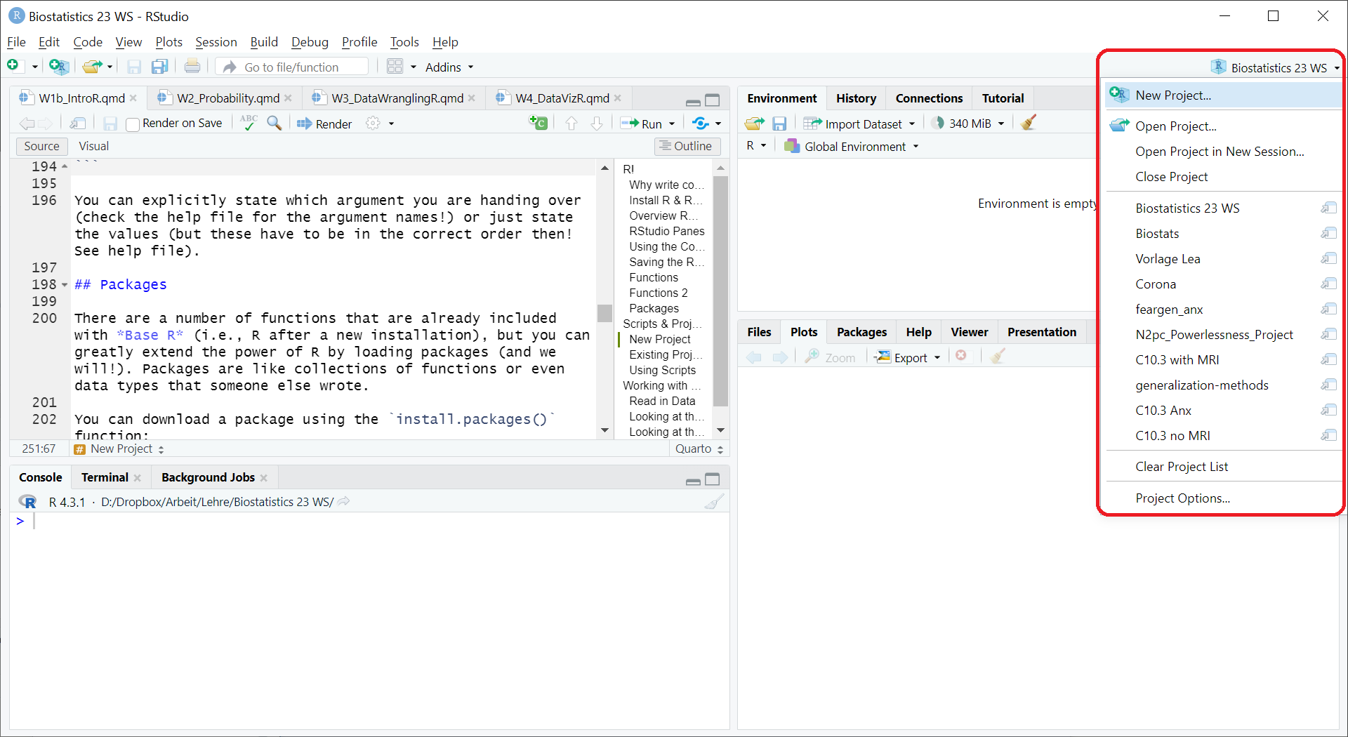
You will find the current project on the top right corner of RStudio
If you click on the current project, you can open new projects by choosing “Open Project” and select the .Rproj file of the project.
You can also just double click on .Rproj files and RStudio will open with the project loaded.
Existing projects
Why Projects
Projects are not only convenient for us (e.g., scripts that we had opened before are re-opened when we open the project), they are also great for reproducibility.
We won’t cover the details here - see the “Further Reading” section of the course page!
Using Scripts
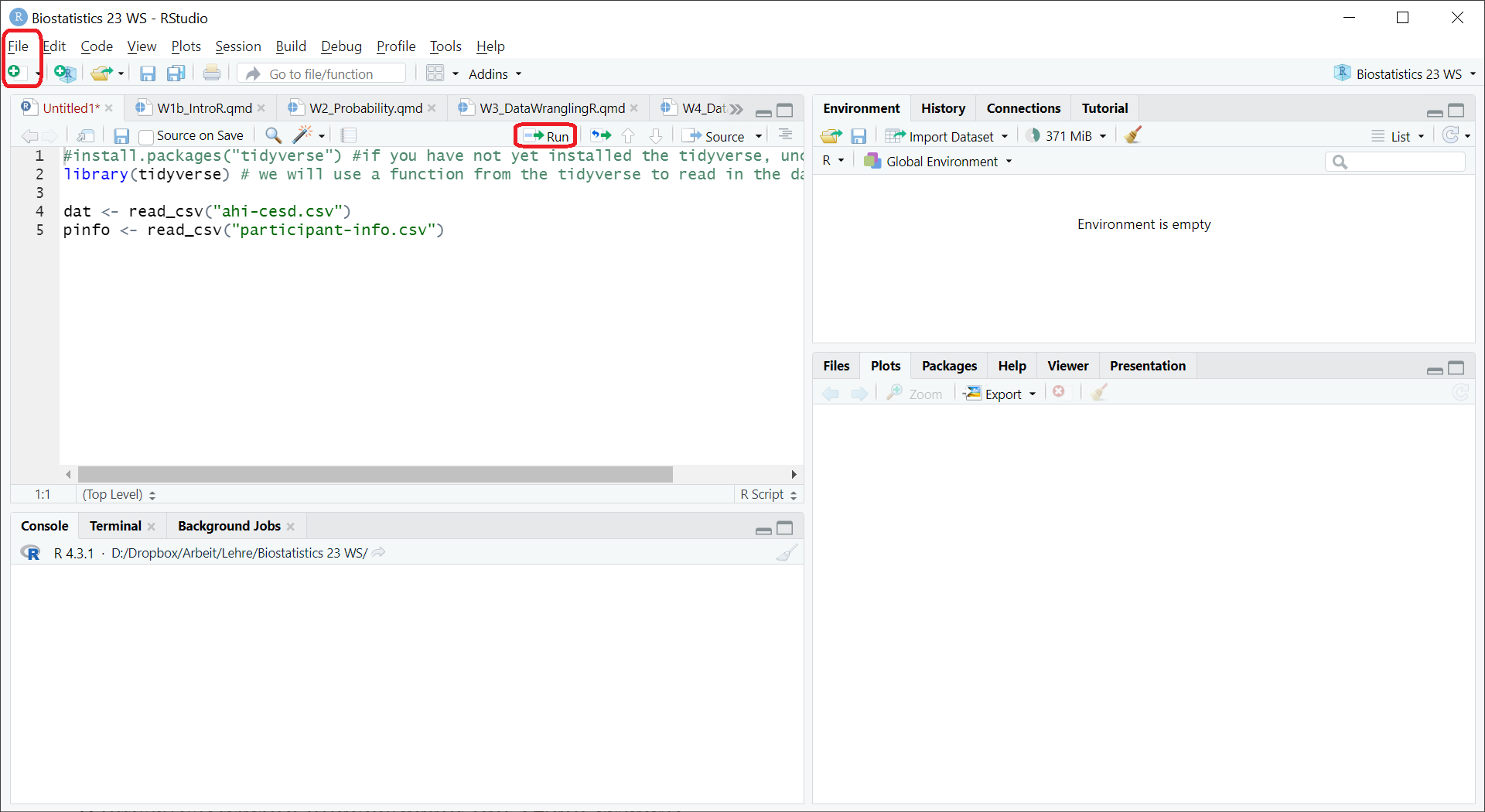
To open a new script, click File\(\to\)New File\(\to\)R Script. (Ctrl + Shift + N)
To run a line of the script, you can either click Run at the top right of the pane or Ctrl + Enter. It will run the code that is highlighted/selected or automatically select the current line (or the complete multi-line command).
To run the whole script/chunk, press Ctrl + Shift + Enter (with full console output) or Ctrl + Shift + S (limited output).
Using scripts
Vectors
So far, we’ve worked with single values; vectors contain several elements.
c(1, 7, 12, 4, 2)
[1] 1 7 12 4 2
c(2, 6.1, 9.234, 1.23)
[1] 2.000 6.100 9.234 1.230
c("hello", "cake", "biscuit")
[1] "hello" "cake" "biscuit"
Vectors always contain the same data type (It’s a bit tricky, but can you see why c(10, "biscuit", 2.31) does not work?).
Vectors are always wrapped in the c() function (“combine”).
But the real fun is that R is “vectorized”, which allows us to do some funny tricks.
Note that this is different from usual “vector math”.
c(1, 2, 5) +1
[1] 2 3 6
c(2, 4, 6) +c(1, 0, 2)
[1] 3 4 8
# Can you spot what happens HERE?!c(2, 4, 6, 5, 0, 0) +c(1, 10)
[1] 3 14 7 15 1 10
Working with real data
Get the data
To read in data files, you need to know which format these files have, e.g. .txt. or .csv files or some other (proprietary) format. There are packages that enable you to read in data of different formats like Excel (.xlsx).
We will use the files from Fundamentals of Quantitative Analysis: ahi-cesd.csv and participant-info.csv. Save these directly in your project folder on your computer (do not open them!).
Did you find the files? Here are the direct links:
library(tidyverse) # we will use a function from the tidyverse to read in the datadat <-read_csv("ahi-cesd.csv")pinfo <-read_csv("participant-info.csv")
Run the code!
Looking at the Data
There are several options to get a glimpse at the data:
Click on dat and pinfo in your Environment.
Type View(dat) into the console or into the script pane and run it.
Run str(dat) or str(pinfo) to get an overview of the data.
Run summary(dat).
Run head(dat), print(dat), or even just dat.
What is the difference between these commands?
Looking at the Data 2
What is the difference to the objects/variables, that you assigned/saved in your Environment earlier and these objects?
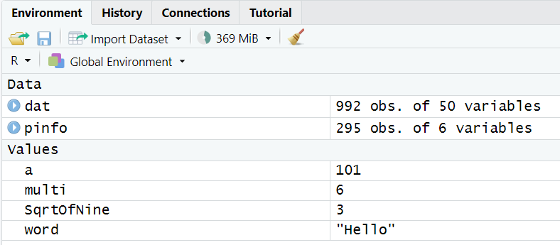
RStudio’s Environment panel
The two objects we just read in are data frames, which are “tables” of data (they can contain entire data sets). The objects we assigned earlier were simpler (single values, or “one-dimensional” vectors).
Data frames usually have several rows and columns. The columns are the variables and the rows are the observations (more about that later).
Questions?
This was the first chapter of this workshop! Do you have any questions?
Comments