2.2 Confidence Intervals
Workshop: “Handling Uncertainty in your Data”
CIs around means
Data preparation
- If you haven’t done so yet: Create an
Rproject for the precision workshop. - Create a script for this part of the workshop (e.g.,
cis.R). - Load the
tidyverse(library(tidyverse)) at the beginning of your script.
Note: We show different packages that help us with confidence interval calculations, some of which may have conflicting functions. This is why in this presentation, we call each package explicitly, e.g., confintr::ci_mean().
Why confidence intervals?
- Goal: indicate precision of a point estimate (e.g., the mean).
- If visualized, it’s often supposed to help with “inference by eye”.
- However, confidence intervals are often misinterpreted (e.g., Hoekstra et al., 2014)
What is a confidence interval?
- Assume we use a 95% CI.
- In the long run, in 95% of our replications, the interval we calculate will contain the true population mean.
- As with any statistical inference: no guarantee! Errors are possible.
- “If a given value is within the interval of a result, the two can be informally assimilated as being comparable.” (Cousineau, 2017)
Confidence interval of the mean
- \(M\) = mean of a set of observations
- \(SE_{M}\) = standard error of the mean
- \(SE_{M} = s/\sqrt n\)
- \(t_{\gamma}\) = multiplier from a Student \(t\) distribution, with d.f. \(n - 1\) and coverage level \(\gamma\) (often 95%)
Briefly: The iris data
Data about the size of three different species of iris flowers.
In R: Confidence interval of the mean
The package confintr offers a variety of functions around confidence intervals. Default here: Student’s \(t\) method.
    Two-sided 95% t confidence interval for the population mean

Sample estimate: 1.326
Confidence interval:
    2.5%    97.5%
1.269799 1.382201
Also available: Wald and bootstrap CIs.
Confidence interval of the mean
- However: very “limited” CI!
- Comparison to a fixed value (e.g., population mean).
- Cannot easily be used to compare different means.
- Useless to compare means of repeated-measures designs.
CIs: comparing groups
- Position of each group mean as well as the relative position of the means are uncertain.
- I.e., SE for the comparison between two means is larger than for the comparison of a mean with a fixed value.
- How much the CI needs to be expanded depends on the variance of each group.
- When the variance is homogeneous across conditions, there is a shortcut: The sum of two equal variances can be calculated by multiplying the common variance by two.
- I.e., the CI must be \(\sqrt2\) (\(\approx\) 1.41) times wider (\(SE_{M} = \sqrt{Var_{SEM}}\)).
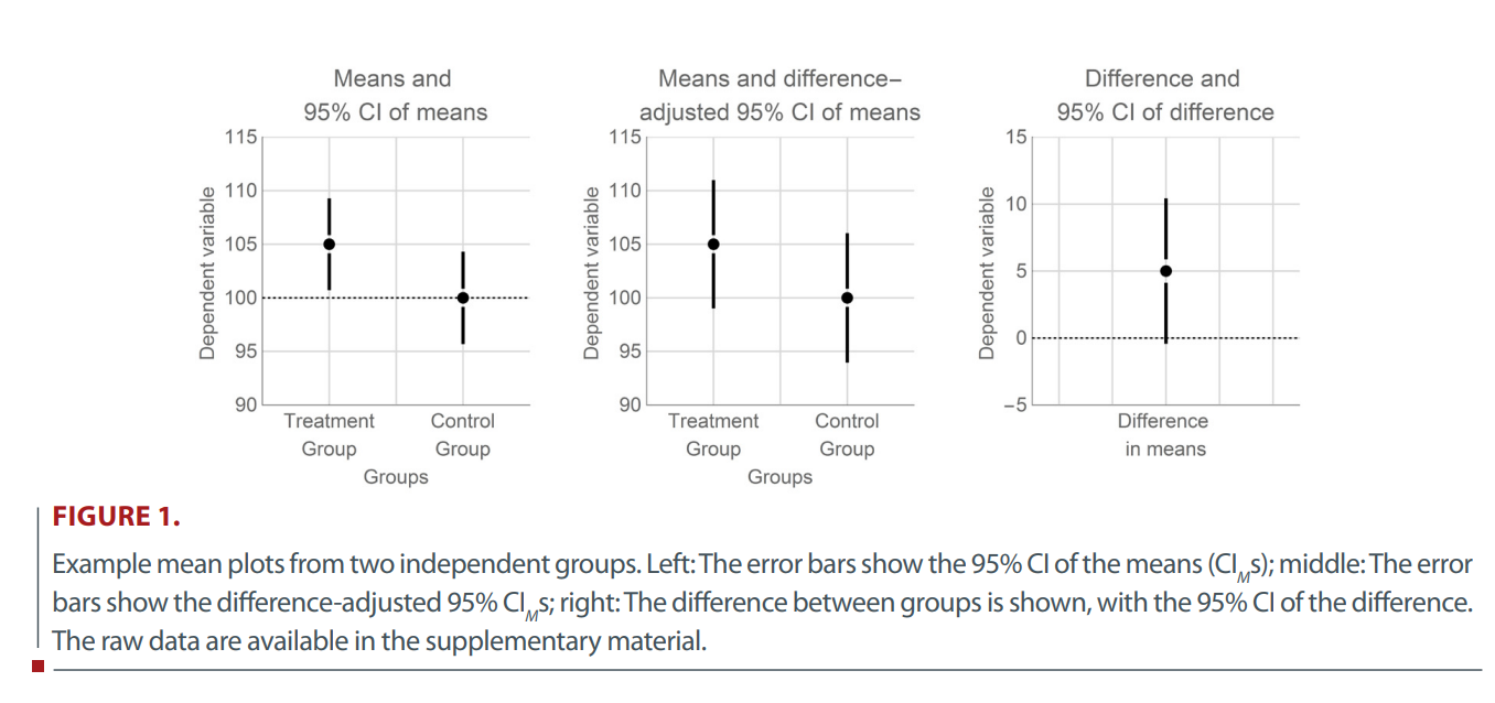
CIs: potential problems when comparing groups
See Cousineau, 2017 - more about data viz later!
In R: custom function
- Sometimes, writing your own custom function gives you the control you need over certain calculations.
In R: custom function - applied
iris %>%
  filter(Species %in% c("setosa", "versicolor")) %>%
  summarise(
    ci_lower = mean(Petal.Width) - se(Petal.Width) * z_CI_t(Petal.Width, .95),
    ci_upper = mean(Petal.Width) + se(Petal.Width) * z_CI_t(Petal.Width, .95),
    .by = Species
  )
Species ci_lower ci_upper
1 setosa 0.2160497 0.2759503
2 versicolor 1.2697993 1.3822007CIs: comparing groups
- Wider CIs for group comparisons, as e.g. suggested by Cousineau (2017).
iris %>%
  filter(Species %in% c("setosa", "versicolor")) %>%
  summarise(
    ci_lower = mean(Petal.Width) - se(Petal.Width) * sqrt(2) * z_CI_t(Petal.Width, .95),
    ci_upper = mean(Petal.Width) + se(Petal.Width) * sqrt(2) * z_CI_t(Petal.Width, .95),
    .by = Species
  )
Species ci_lower ci_upper
1 setosa 0.2036439 0.2883561
2 versicolor 1.2465202 1.4054798- Attention! Assumes equal variance!
- Even though here, we use the mean and SD/SE of each group (not e.g. the pooled SD).
CIs: difference of means
- If possible, the most elegant way is to report/plot the CI for the difference in means.
with(
  iris,
  confintr::ci_mean_diff(
    Petal.Width[Species == "versicolor"],
    Petal.Width[Species == "setosa"]
  )
)
    Two-sided 95% t confidence interval for the population value of
    mean(x)-mean(y)

Sample estimate: 1.08
Confidence interval:
    2.5%    97.5%
1.016867 1.143133 - Not pipe-friendly, if that’s important for you.
- Careful! Not for within-subjects comparisons!
CIs: difference of means
- Looks familiar? Part of the
t.test()output by default!
    Welch Two Sample t-test

data:  Petal.Width[Species == "versicolor"] and Petal.Width[Species == "setosa"]
t = 34.08, df = 74.755, p-value < 2.2e-16
alternative hypothesis: true difference in means is not equal to 0
95 percent confidence interval:
 1.016867 1.143133
sample estimates:
mean of x mean of y
    1.326     0.246
CIs: difference of means
- Looks familiar? Part of the
t.test()output by default! - Can be accessed like this:
What about within-subject designs?
- Repeated measures are typically correlated, which makes it possible to evaluate the difference between means more precisely.
- I.e., we adjust the width of the CI based on the correlation between measures.
- The difference between the two means is estimated as if we had a larger (independent) sample.
Note that we still are comparing two means, so as before, the CI is “difference adjusted” using \(\sqrt2\).
Briefly: the fhch2010 data
- Data from Freeman, Heathcote, Chalmers, & Hockley (2010), included in
afex. - Lexical decision and word naming latencies for 300 words and 300 nonwords.
- For simplicity, we’re only interested in the task (word naming or lexical decision; between subjects) and the stimulus (word or nonword).
  id   task stimulus density frequency length   item    rt      log_rt correct
1 N1 naming     word    high       low      6 potted 1.091  0.08709471    TRUE
2 N1 naming     word     low      high      6 engine 0.876 -0.13238919    TRUE
3 N1 naming     word     low      high      5  ideal 0.710 -0.34249031    TRUE
4 N1 naming  nonword    high      high      5  uares 1.210  0.19062036    TRUE
5 N1 naming  nonword     low      high      4   xazz 0.843 -0.17078832    TRUE
6 N1 naming word high high 4 fill 0.785 -0.24207156 TRUECIs for within-subject designs
The measures are highly correlated :-)
fhch2010_summary_wf <-
  fhch2010_summary %>%
  pivot_wider(
    id_cols = id,
    names_from = stimulus,
    values_from = rt
  )

fhch2010_summary_wf %>%
  rstatix::cor_test(word, nonword)
# A tibble: 1 × 8
var1 var2 cor statistic p conf.low conf.high method
<chr> <chr> <dbl> <dbl> <dbl> <dbl> <dbl> <chr>
1 word nonword 0.8 8.67 5.40e-11 0.658 0.884 PearsonCIs for within-subject designs
# without adjusting
fhch2010_summary %>%
  summarise(
    ci_lower = mean(rt) - se(rt) * sqrt(2) * z_CI_t(rt, .95),
    ci_upper = mean(rt) + se(rt) * sqrt(2) * z_CI_t(rt, .95),
    .by = stimulus
  )
stimulus ci_lower ci_upper
1 word 0.8119932 1.056787
2 nonword 0.9912777 1.206521# adjust for correlation
word_cor <- cor.test(fhch2010_summary_wf$word, fhch2010_summary_wf$nonword)
fhch2010_summary %>%
summarise(
ci_lower = mean(rt) - se(rt) * sqrt(1 - word_cor$estimate) * sqrt(2) * z_CI_t(rt, .95),
ci_upper = mean(rt) + se(rt) * sqrt(1 - word_cor$estimate) * sqrt(2) * z_CI_t(rt, .95),
.by = stimulus
) stimulus ci_lower ci_upper
1 word 0.8793337 0.989447
2 nonword 1.0504891 1.147310CIs for differences in means in within-subject designs
As before, the \(t\)-test will give us a CI for the difference in means:
with(
  fhch2010_summary,
  t.test(
    rt[stimulus == "word"],
    rt[stimulus == "nonword"],
    paired = TRUE
  )
)
    Paired t-test

data:  rt[stimulus == "word"] and rt[stimulus == "nonword"]
t = -6.2944, df = 44, p-value = 1.245e-07
alternative hypothesis: true mean difference is not equal to 0
95 percent confidence interval:
 -0.2171825 -0.1118359
sample estimates:
mean difference
-0.1645092 CIs: caveats
- Assumptions: normally distributed means, homogeneity of variances, sphericity (repeated measures)
- Mixed designs: Difficult! You will probably need to choose between between-subject or within-subject CIs (depending on your comparisons of interest); see upcoming data viz part!
- Most importantly: Be transparent! Describe how you calculated your CIs and what they are for!
CIs around effect sizes
Cohen’s d
- Also possible to report CIs on effect size estimates; different methods of calculating the desired CIs for different measures exist (beyond the scope of this workshop).
- E.g.,
cohens_d()from the packageeffectsize: “CIs are estimated using the noncentrality parameter method (also called the ‘pivot method’)”; see further details at
?effectsize::cohens_d().
rstatix: pipe-friendly t-test
rstatixoffers pipe-friendly statistical tests, and also calculates CIs.detailed = TRUEwill give us confidence estimates for our \(t\)-test.
iris %>%
  filter(Species %in% c("setosa", "versicolor")) %>%
  rstatix::t_test(Petal.Width ~ Species, detailed = TRUE) %>%
  select(contains("estimate"), statistic:conf.high) #reduce output for slide
# A tibble: 1 × 8
estimate estimate1 estimate2 statistic p df conf.low conf.high
<dbl> <dbl> <dbl> <dbl> <dbl> <dbl> <dbl> <dbl>
1 -1.08 0.246 1.33 -34.1 2.72e-47 74.8 -1.14 -1.02rstatix: pipe-friendly Cohen’s d
- Also includes a pipe-friendly version of Cohen’s d.
- Careful: CIs are bootstrapped (hence the small discrepancy to the output of
effectsizeearlier)
iris %>%
  filter(Species %in% c("setosa", "versicolor")) %>%
  rstatix::cohens_d(Petal.Width ~ Species, ci = TRUE)
# A tibble: 1 × 9
.y. group1 group2 effsize n1 n2 conf.low conf.high magnitude
* <chr> <chr> <chr> <dbl> <int> <int> <dbl> <dbl> <ord>
1 Petal.Width setosa versicolor -6.82 50 50 -8.31 -5.95 large Correlations: apa
Option 1: Using the apa package.
Correlations: rstatix
Option 2: Using the rstatix package.
iris %>%
  group_by(Species) %>%
  rstatix::cor_test(Petal.Width, Petal.Length) #implicitly ungroups the data
# A tibble: 3 × 9
Species var1 var2 cor statistic p conf.low conf.high method
<fct> <chr> <chr> <dbl> <dbl> <dbl> <dbl> <dbl> <chr>
1 setosa Petal.Wid… Peta… 0.33 2.44 1.86e- 2 0.0587 0.558 Pears…
2 versicolor Petal.Wid… Peta… 0.79 8.83 1.27e-11 0.651 0.874 Pears…
3 virginica Petal.Wid… Peta… 0.32 2.36 2.25e- 2 0.0481 0.551 Pears…Note: Only gives rounded values …
ANOVAs
aov_words <-
  aov_ez(
    id = "id",
    dv = "rt",
    data = fhch2010_summary,
    between = "task",
    within = "stimulus",
    # we want to report partial eta² ("pes"), and include the intercept in the output table ...
    anova_table = list(es = "pes", intercept = TRUE)
  )

aov_words
Anova Table (Type 3 tests)
Response: rt
Effect df MSE F pes p.value
1 (Intercept) 1, 43 0.10 904.33 *** .955 <.001
2 task 1, 43 0.10 15.76 *** .268 <.001
3 stimulus 1, 43 0.01 77.24 *** .642 <.001
4 task:stimulus 1, 43 0.01 31.89 *** .426 <.001
---
Signif. codes: 0 '***' 0.001 '**' 0.01 '*' 0.05 '+' 0.1 ' ' 1CI around partial eta²
In principle, apaTables offers a function for CIs around \(\eta_p^2\) …
# e.g., for our task effect
apaTables::get.ci.partial.eta.squared(
  F.value = 15.76, df1 = 1, df2 = 43, conf.level = .95
)
$LL
[1] 0.06851017
$UL
[1] 0.4511011… but it would be tedious to copy these values.
CI around partial eta²
A little clunky function that can be applied to afex tables:
peta.ci <-
  function(anova_table, conf.level = .9) { # 90% CIs are recommended for partial eta² (https://daniellakens.blogspot.com/2014/06/calculating-confidence-intervals-for.html#:~:text=Why%20should%20you%20report%2090%25%20CI%20for%20eta%2Dsquared%3F)

    result <-
      apply(anova_table, 1, function(x) {
        ci <-
          apaTables::get.ci.partial.eta.squared(
            F.value = x["F"], df1 = x["num Df"], df2 = x["den Df"], conf.level = conf.level
          )

        return(setNames(c(ci$LL, ci$UL), c("LL", "UL")))
      }) %>%
      t() %>%
      as.data.frame()

    result$conf.level <- conf.level

    return(result)
  }
CI around partial eta²
The result of custom function that applies the apaTables function to our entire ANOVA table:
                      LL        UL conf.level
(Intercept)   0.92985360 0.9656284        0.9
task          0.09399555 0.4224818        0.9
stimulus      0.48335736 0.7294335        0.9
task:stimulus 0.23280549 0.5584355        0.9
Also see this blogpost by Daniel Lakens from 2014 about CIs for \(\eta_p^2\).
Thanks!
Learning objectives:
- Understand what different versions of CIs exist, and which one you need for your data.
- Apply different functions in
R(and write custom ones if needed) to report CIs around means, and common effect size estimates.
Next: Visualizing uncertainty