09 Statistical Analyses in R

Julius-Maximilians-University Würzburg
Course: “Biostatistics”
Translational Neuroscience

Dr. Mario Reutter (slides adapted from Dr. Lea Hildebrandt)

Kinds of Statistical Analyses

Last session, we have heard about Chi² tests, t-tests, correlations, and ANOVA.

Today we will apply them in R.

An important part of today will be: How do I wrangle the data such that it fits to the functions available in R?

Set Up

1. Open RStudio and load your Biostats R project. Create a new script called DataAnalysis1.R.

2. Install and load new packages you’ll need:

library(car)
library(apa)
library(effectsize)
library(confintr)
library(afex)
library(performance)
library(emmeans)
library(pwr)
library(lsr)
library(report)
library(tidyverse)

Activity 1

Which test would you choose if you wanted to test whether a variable is differently distributed between groups? More specifically, the variable contains counts.

Let’s say we have tested 20 mice and want to know whether they pressed the blue, green, or red lever more often than by chance. This is how often the mice pressed each lever: Blue = 5, Green = 4, Red = 11

We would run a (one-sample) Chi²-test!

Remember that in a Chi²-test, we would compare observed to expected counts:

\[ \chi^2 = \sum\frac{(Observed - Expected)^2}{Expected} \]

One Sample Chi²-Test

library(tidyverse) 

# Input data into R
lever_presses <- tibble(levers=c(rep("blue", 5), rep("green", 4), rep("red", 11))) %>% #data in usual format
  count(levers) #convert to a frequency table (most useful for tables)
lever_presses_wide <- lever_presses %>% 
  pivot_wider(names_from="levers", values_from="n") #wide format (needed for chisq.test function)

# run Chi² test
chi2_lever <- chisq.test(lever_presses_wide) 
#chi2_lever <- chisq.test(tibble(blue=5, green=4, red=11)) #enter data directly as summary table

chi2_lever %>% apa::chisq_apa() #output results

chi^2(2) = 4.30, p = .116

One Sample Chi²-Test: Expected Values & Residuals

# add expected count and residuals to data
lever_presses %>% mutate(expected = chi2_lever$expected, 
                         diff = n - expected,
                         residuals = chi2_lever$residuals)

# A tibble: 3 × 5
  levers     n expected  diff residuals
  <chr>  <int>    <dbl> <dbl>     <dbl>
1 blue       5     6.67 -1.67    -0.645
2 green      4     6.67 -2.67    -1.03 
3 red       11     6.67  4.33     1.68 

Is sample size not important for significance here? \[\chi^2 = \sum\frac{(Observed - Expected)^2}{Expected}\] More observations => easier to see greater absolute difference between observed and expected values => gets squared and therefore “outcompetes” denominator (what about expected reductions in sampling error?)

Chi²-Test 2

We can also run a Chi²-test for two variables, such as if we want to know whether the lever press distributions differ between two (or more) groups.

Let’s say we have a treatment and a control group and we record the different lever presses:

Group	Blue	Green	Red	Totals
Treatment	3	12	5	20
Control	5	4	11	20
Totals	8	16	16	40

Remember: We use the assumption of independence to calculate the expected values.

lever_presses2 = tibble(group="treatment", blue=3, green=12, red=5) %>% 
  bind_rows(tibble(group="control", blue=5, green=4, red=11)) #clearest way to manually input data
#for long data, you create the frequency table identically to previous slide but with: count(group, levers)

chisq.test(lever_presses2 %>% column_to_rownames("group")) %>% apa::chisq_apa()

chi^2(2) = 6.75, p = .034

Assumptions of Chi²-Tests

• Random sample

• Categorical variables, i.e., counts within (combinations of) groups

• Expected cell count: >5 counts per cell

• Independence: Each observation is independent of the others, e.g. there are no repeated measurements/paired data (within-subjects data are correlated!)

In the case of the last analysis, we got a warning because the expected cell sizes were too small. In this case, it is better to use Fisher’s exact test:

fisher.test(lever_presses2 %>% column_to_rownames("group"))

    Fisher's Exact Test for Count Data

data:  lever_presses2 %>% column_to_rownames("group")
p-value = 0.04168
alternative hypothesis: two.sided

Activity 2

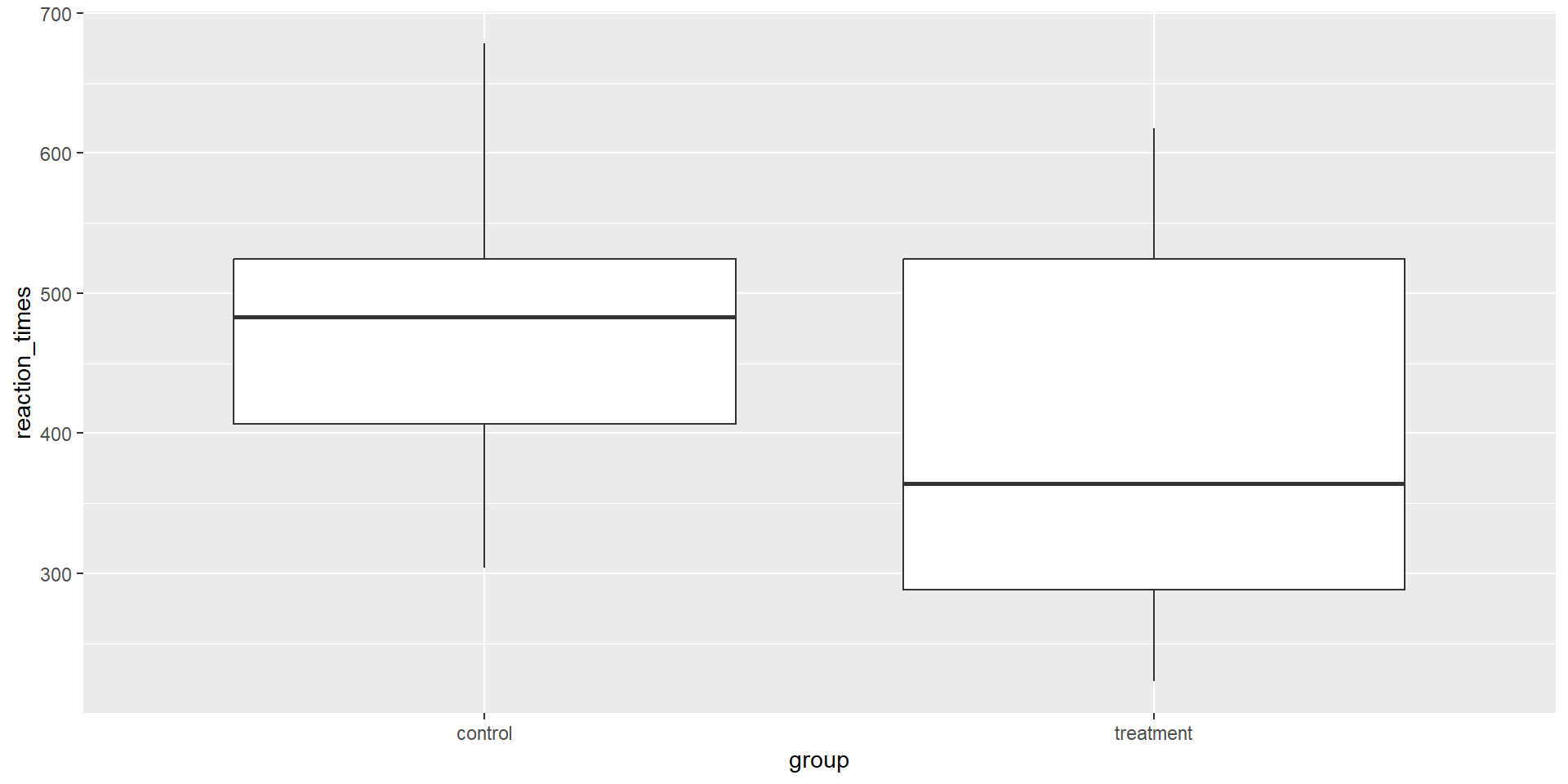
Now imagine you want to compare reaction times of the lever presses of the two groups of mice. You expect that those in the treatment group respond faster than those in the control group. Which statistical test would you use?

Hint: We now have two independent groups and a continuous dependent variable (reaction times).

⇒ An (independent samples) t-test!

t-test setup

To run a t-Test, let’s first simulate data. What happens here?

set.seed(31415)
sim_data_t <- tibble(
  group = rep(c("treatment", "control"), each=20),
  reaction_times = c(rnorm(20, 400, 100), rnorm(20, 450, 100))) #poorly documented code for practice

t-Test: Formula Notation

We can use the formula notation to run the t-test. This notation usually looks like this:
dependent variable ~ independent variable.

Replace the NULLs:

t.test(NULL ~ NULL,
       data = NULL,
       alternative = NULL,
       paired = NULL) 

t-Test: Formula Notation

We can use the formula notation to run the t-test. This notation usually looks like this:
dependent variable ~ independent variable.

Replace the NULLs:

t.test(reaction_times ~ group,
       data = sim_data_t,
       alternative = "greater", #depends on ALPHABETICAL order of groups in data! (if not coded as factor)
       #paired = FALSE # this is the default, so no need to specify it
)

    Welch Two Sample t-test

data:  reaction_times by group
t = 1.9841, df = 34.42, p-value = 0.02763
alternative hypothesis: true difference in means between group control and group treatment is greater than 0
95 percent confidence interval:
 10.02639      Inf
sample estimates:
  mean in group control mean in group treatment 
               468.0592                400.3289 

t-Test: Formula Notation

t.test(reaction_times ~ group,
       data = sim_data_t,
       alternative = "greater", #depends on ALPHABETICAL order of groups in data! (if not coded as factor)
       #paired = FALSE # this is the default, so no need to specify it
)

    Welch Two Sample t-test

data:  reaction_times by group
t = 1.9841, df = 34.42, p-value = 0.02763
alternative hypothesis: true difference in means between group control and group treatment is greater than 0
95 percent confidence interval:
 10.02639      Inf
sample estimates:
  mean in group control mean in group treatment 
               468.0592                400.3289 

As you can see in the output, R automatically chose to run Welch’s t-test, which does not assume homogeneity of variance in contrast to Student’s t-test. For the latter, you can add the function parameter var.equal = TRUE

When changing the name “treatment” to “a”, the results change:

t.test(reaction_times ~ group,
       data = sim_data_t %>% mutate(group = ifelse(group=="treatment", "a", group)),
       alternative = "greater", #depends on order of groups in data! 1st group > 2nd group
       var.equal = TRUE) %>% apa::t_apa()

t(38) = -1.98, p = .973, d = -0.63

t-Test with filter

You can also supply two vectors of numerical values for the groups:

t.test(x = sim_data_t %>% filter(group=="treatment") %>% pull(reaction_times),
       y = sim_data_t %>% filter(group=="control") %>% pull(reaction_times),
       alternative = "less") #more intuitive now because you can filter for treatment first

    Welch Two Sample t-test

data:  sim_data_t %>% filter(group == "treatment") %>% pull(reaction_times) and sim_data_t %>% filter(group == "control") %>% pull(reaction_times)
t = -1.9841, df = 34.42, p-value = 0.02763
alternative hypothesis: true difference in means is less than 0
95 percent confidence interval:
      -Inf -10.02639
sample estimates:
mean of x mean of y 
 400.3289  468.0592 

This makes it easier to think about the direction of the alternative hypothesis because you choose which group is considered first.

t-Test: apa package

More useful output with apa package (only for Student’s t-tests):

t.test(x = sim_data_t %>% filter(group=="treatment") %>% pull(reaction_times),
       y = sim_data_t %>% filter(group=="control") %>% pull(reaction_times),
       alternative = "less", 
       var.equal = TRUE) %>% 
  apa::t_apa(es_ci = TRUE) #optional: confidence interval around effect size

t(38) = -1.98, p = .027, d = -0.63 [-1.26; 0.01]

t-Test: paired samples

For paired t-tests, you have to work with the wide format of data (advantage: missing values become explicit):

sim_data_t_wide = sim_data_t %>% mutate(subject=rep.int(1:(n()/2), 2)) %>% 
  pivot_wider(names_from="group", values_from="reaction_times", id_cols = subject)
t.test(x = sim_data_t_wide %>% pull(treatment),
       y = sim_data_t_wide %>% pull(control),
       alternative = "less", 
       paired = TRUE) %>% 
  apa::t_apa(es_ci = TRUE) #optional: confidence interval around effect size

t(19) = -1.98, p = .031, d = -0.44 [-0.90; 0.02]

You can also use the wide format for the independent samples t-test (instead of formula notation or filtering). You choose 😊.

Assumptions of t-Tests

Before we run a t-test, we also want to check the assumptions for violations:

• The dependent variable is continuous (otherwise: chi²-test)

• The data are independent (otherwise: paired sample t-test)

• The variance between the groups is homogeneous (only for Student’s t-test, R uses Welch’s test by default)

• The residuals are normally distributed for each group (otherwise: wilcox.test)

Oftentimes, the last assumption is misquoted as: “The dependent variable needs to be normally distributed”.
In fact, only its sampling distribution needs to be (blue vs. grey distribution in the lecture on sampling [direct link]), which will always be the case for big enough samples due to the central limit theorem.

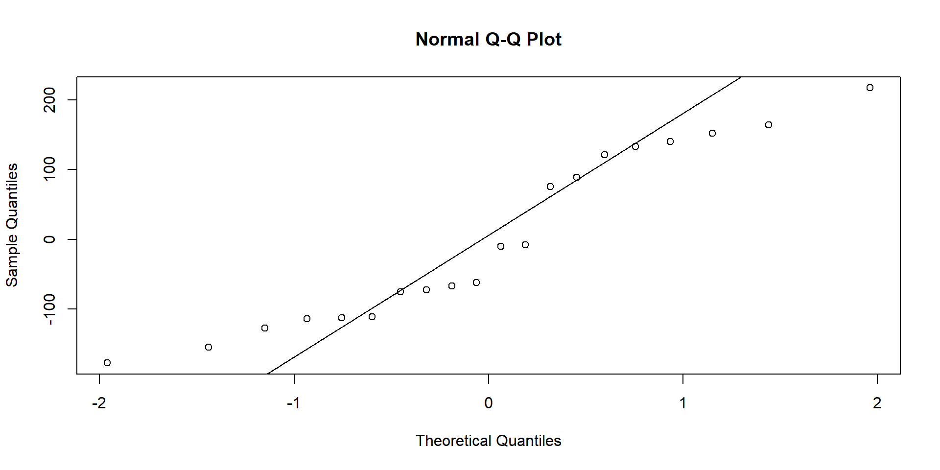
Assumptions of t-Tests: Normality

Test for normality of residuals (for both groups separately): If points fall along the line nicely, assumption is met.

Treatment group:

treatment <- sim_data_t %>%
  filter(group == "treatment") %>%
  mutate(group_resid = 
           reaction_times - mean(reaction_times)) %>%
  pull(group_resid)

#base R QQ plot
qqnorm(treatment)
qqline(treatment)

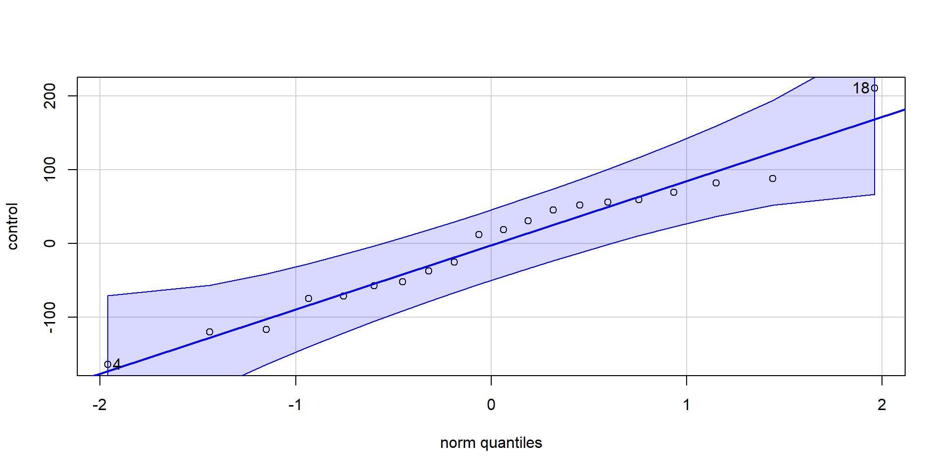
Assumptions of t-Tests: Normality

Test for normality of residuals (for both groups separately): If points fall along the line nicely, assumption is met.

Control group group:

control <- sim_data_t %>%
  filter(group == "control") %>%
  mutate(group_resid = 
           reaction_times - mean(reaction_times)) %>%
  pull(group_resid)

#car's version highlighting (and returning) problematic values
car::qqPlot(control)

[1] 18  4

Assumptions of t-Tests: Normality

Alternatively, we can also run a Shapiro-Wilk test to check for deviations from normality:

shapiro.test(x = treatment)

    Shapiro-Wilk normality test

data:  treatment
W = 0.91403, p-value = 0.0761

shapiro.test(x = control)

    Shapiro-Wilk normality test

data:  control
W = 0.96812, p-value = 0.7147

If the test is non-significant, then we can conclude that normality of residuals is not violated.

⇒ Shapiro-Wilk tests for significant deviations from normality.

1. Transform your data to try and normalise the distribution. Not usually recommended these days but some still use it.
2. Use a non-parametric test. The non-parametric equivalent of the independent t-test is the Mann-Whitney and the equivalent of the paired-samples t-test is the Wilcoxon signed-ranks test. Though more modern permutation tests are better.
3. Do nothing. Delacre, Lakens & Leys, 2017 argue that with a large enough sample (>30), the Welch test is robust to deviations from assumptions. With very large samples normality is even less of an issue, so design studies with large samples.

Optional Activity: Paired Samples t-Test

Sometimes you have dependent data: These data are somehow correlated, e.g. they belong to the same subject (that you measured repeatedly across a within-subject manipulation).

In this case, you would use a paired-samples t-test.

Let’s run such a t-test with real data. We’ll use the Mehr Song and Spelke 2016 Experiment 1.csv file (note that this is not a good file name!).

Mehr, Song, & Spelke (2016)

In this dataset, the authors examined whether infants exposed to certain songs would recognize strangers singing these lullabies as part of their social group. Parents sang certain lullabies to their infants for 1-2 weeks. During the experiment, the infants looked at videos of two strangers: First the strangers were just smiling (baseline phase), then they would sing either the familiar or an unfamiliar lullaby. Finally, the infants again saw the videos of the strangers smiling (test phase). Eye-tracking (duration looked at each stranger) was measured.

Load the file into your Environment. Run the code and explain what happens:

gaze <- read_csv("Mehr Song and Spelke 2016 Experiment 1.csv") %>%
  filter(exp1 == 1) %>%
  rename(baseline = Baseline_Proportion_Gaze_to_Singer,
         test = Test_Proportion_Gaze_to_Singer) %>% 
  select(id, baseline, test)

Assumptions of the Paired-Samples t-Test

1. The data are continuous.

2. All participants should appear in both conditions/groups.

3. The residuals are normally distributed.

A paired-samples t-test actually tests whether the difference between two measurements is significantly different from 0 (= no difference/effect).

In our example data, this means that the test values are subtracted from the baseline values, and this difference is used as data.

To test the assumption that residuals are normally distributed, we thus calculate the residuals as follow:

gaze_residual <- gaze %>%
  mutate(diff = baseline - test) %>%
  mutate(group_resid = diff - mean(diff))

Assumptions of the Paired-Samples t-Test

[1] 22 29

    Shapiro-Wilk normality test

data:  gaze_residual$group_resid
W = 0.97818, p-value = 0.7451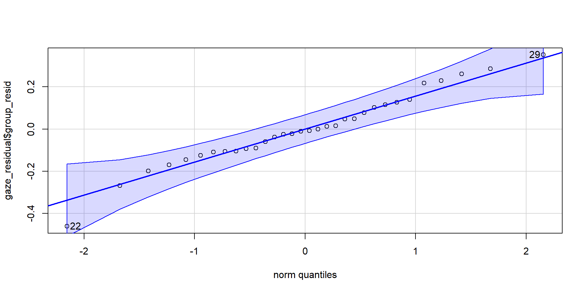

Descriptives & Visualization

For the visualization, we need the data in long format (this is identical for between-subject groups):

gaze_tidy <- gaze %>%
  pivot_longer(names_to = "phase", 
               values_to = "looking_time", 
               cols = c(baseline, test))

# boxplot
gaze_tidy %>% 
  ggplot(aes(x=phase, y=looking_time)) +
  geom_boxplot()

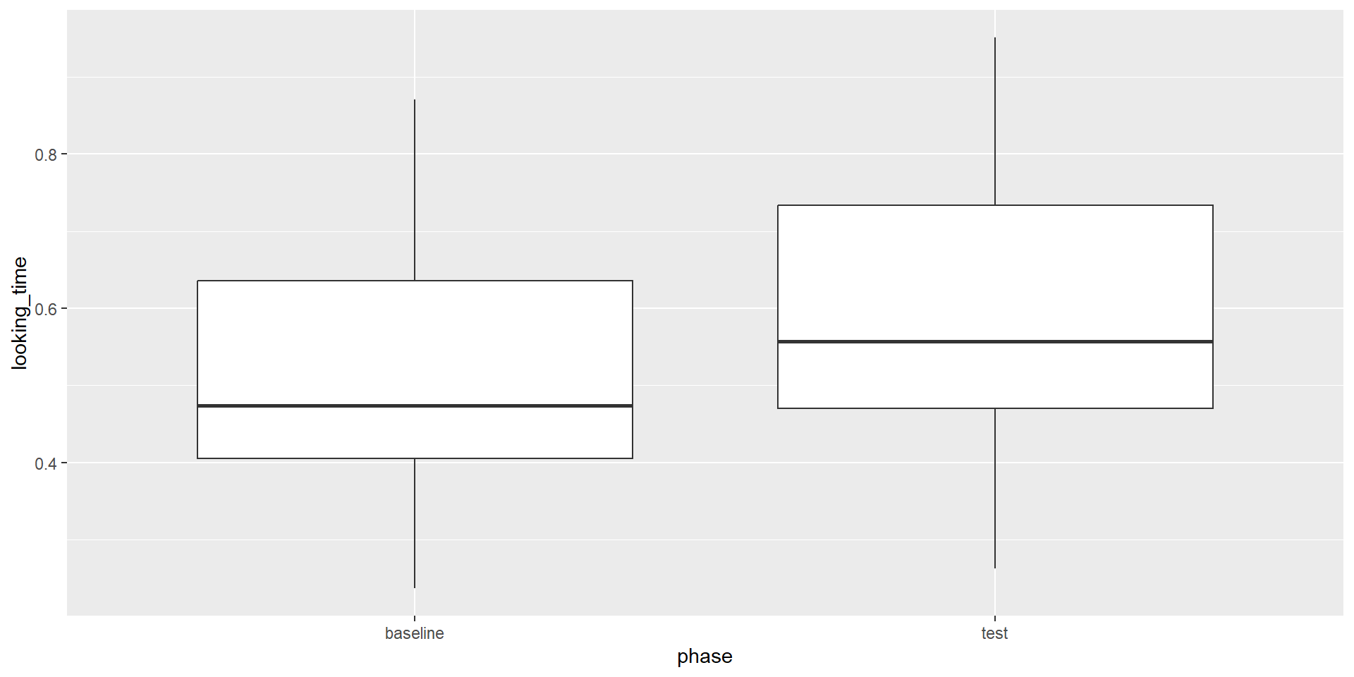
We can also calculate the means and SDs per phase:

gaze_tidy %>% 
  summarize(.by = phase,
            mean_looking = mean(looking_time),
            sd_looking = sd(looking_time),
            n = n())

# A tibble: 2 × 4
  phase    mean_looking sd_looking     n
  <chr>           <dbl>      <dbl> <int>
1 baseline        0.521      0.177    32
2 test            0.593      0.179    32

Paired Samples t-Test in R

Any ideas how you would specify the paired samples t-test in R?

with(gaze, t.test(x = NULL, y = NULL,
                  paired = NULL,
                  alternative = NULL))

with(gaze, t.test(x = baseline, y = test,
                  paired = TRUE,
                  alternative = "two.sided"))

    Paired t-test

data:  baseline and test
t = -2.4164, df = 31, p-value = 0.02175
alternative hypothesis: true mean difference is not equal to 0
95 percent confidence interval:
 -0.13349698 -0.01129217
sample estimates:
mean difference 
    -0.07239458 

Effect Size for the t-Test

You can (and should!) of course calculate and report effect sizes for your test statistics to get an impression of how practically relevant the effect is.

For the t-tests, you would calculate Cohen’s d (e.g., using the effectsize package):

with(gaze, effectsize::cohens_d(baseline, test, paired = TRUE))

Cohen's d |         95% CI
--------------------------
-0.43     | [-0.79, -0.06]

Or just use the apa package and you get everything in one go:

with(gaze, #the with function allows to call columns as if they were variables (but pipe function doesn't work with it)
     t.test(baseline, test, paired = TRUE)) %>% 
  apa::t_apa(es_ci = TRUE)

t(31) = -2.42, p = .022, d = -0.43 [-0.79; -0.06]

Summary: Optional Activity

• Most things are similar between independent and dependent sample t-tests

• Make sure to include paired = TRUE for repeated measures to get correct results

• Recommendation: Use apa::t_apa() with es.ci = TRUE to get (most of) the information you need

• It is often a good idea to also report means and standard deviations per group
  (summarize with .by argument)

• Plotting: Unfortunately, (between subjects) confidence intervals are not diagnostic for the significance of dependent samples. Instead, we need the confidence interval around the paired differences (i.e., the within subject changes).

Kinds of Error Variance in paired samples

Use Notes Canvas (paint brush icon on bottom left) to draw worst possibility of paired differences in “Raw Data” and resulting increase in within-subjects error variance while between-subjects variance remains fixed.

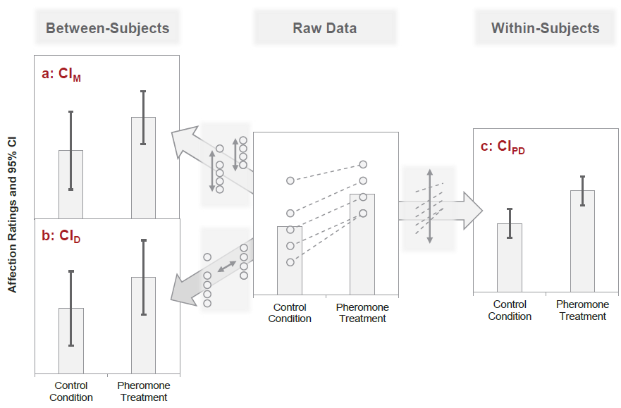
Pfister & Janczyk (2013), Fig. 1

Correlation: Preparation

If we have two continuous variables, we can look at their relationship using correlation. In the data you just used, we have two continuous variables: the repeated measures of gaze.

If you skipped the previous activity, here is what you need:

1. Download Mehr Song and Spelke 2016 Experiment 1.csv (download button near the top right) into your project folder and

2. run this code:

gaze <- read_csv("Mehr Song and Spelke 2016 Experiment 1.csv") %>%
  filter(exp1 == 1) %>%
  rename(baseline = Baseline_Proportion_Gaze_to_Singer,
         test = Test_Proportion_Gaze_to_Singer) %>% 
  select(id, baseline, test)

Correlation Test

We might be interested in whether there is a relationship between the two measures of gaze, i.e., whether those children who looked at the stranger more at baseline would also look more at the follow-up test (here: indicating stability of preferences).

Similar to the paired t-Test, the continuous variables are also “paired” within subjects. Thus, we can use a similar syntax to the previous optional activity of the paired t-test:

cor.test(x = gaze %>% pull(baseline), 
         y = gaze %>% pull(test), 
         method = "pearson", #default
         alternative = "two.sided") %>% #default
  apa::cor_apa(r_ci = TRUE)

r(30) = .55 [.24; .75], p = .001

Note: We don’t have to indicate paired = TRUE because correlations only work for paired values.

We mainly use this dataset so that you don’t have to load another one, but in practice you would either run a t-test or a correlation, not necessarily both!

The t-tests answers whether there is a change across all participants between the two time points, the correlation answers the question whether those who score high at one time point would also score high at the next (regardless of overall level).

Correlations: Write Up

You can even use report() to get an automatic suggestion of how to report the results (works with a lot of different models!).

library(report)
with(gaze, cor.test(x = baseline, 
                    y = test, 
                    method = "pearson", 
                    alternative = "two.sided")) %>% 
  report()

Effect sizes were labelled following Funder's (2019) recommendations.

The Pearson's product-moment correlation between baseline and test is positive,
statistically significant, and very large (r = 0.55, 95% CI [0.24, 0.75], t(30)
= 3.57, p = 0.001)

Who wants to write a package that inputs data & analysis results into ChatGPT? :D

Correlations: Notes

There are also some assumptions that need to be checked:

1. Are the data continuous? (for ordinal values: Spearman’s rho)

2. Is there a data point for each participant on both variables? (paired values)

3. Are the residuals normally distributed?

4. Does the relationship between variables appear linear?

5. Does the spread have homoscedasticity? (Variance of residuals should be constant across x-axis)
   Note: This is very hard to judge by eye and is not the same as the confidence band around the regression line to show constant width. In fact, the latter will always be larger near the ends of the regression line due to how it is computed.

Please see the text book for how to test these assumptions.

You should - as always - also report the descriptive statistics (such as mean and SD of both variables).

You can also report and visualize multiple correlations at once, using a scatterplot matrix or heatmaps. Check out e.g. the corrplot package!

Activity 3

What if we have more than two groups and/or more than one variable? For example, what if we have one variable treatment (with the factor levels treatment 1, treatment 2, and control) and possibly another variable called timepoint (baseline, post-test)?

Which statistical test could we use?

We would possibly run an ANOVA!

If we have only one factor (e.g. treatment with three factor levels), we would do a (one-way) ANOVA.
If we have more than one factor but only between-subjects variables, we would run an ANOVA with interactions (see lecture 10).
If we have at least one within-subjects factor, we would run a repeated measures (or mixed effects) ANOVA.

The names are only there for historical reasons. With the right R packages, we only have to ask ourselves if a variable changes between subjects or within subjects.

Due to their potency and wide-spread use, we will cover ANOVAs even more next time in the context of the linear model.

we will today only look at one-way anovas! Next time we will cover the case when we have more than one IV/predictor!

One-Way ANOVA

For this activity, we will use data from a study about memory of traumatic events (see the textbook for details). In short, the authors of the paper were interested to find out whether:

reconsolidation - the process during which memories become malleable when recalled - can be blocked using a cognitive task and whether such an approach can reduce these unbidden intrusions.

1. Download the data James Holmes_Expt 2_DATA.csv. This time, put it in a subfolder of your project called “Data”.

2. Add a column to the dataframe called subject that equals the row_number(), which will act as a participant ID.

3. rename(): Days_One_to_Seven_Image_Based_Intrusions_in_Intrusion_Diary to intrusions.

4. Select only the columns subject, Condition and intrusions.

5. Change the variable Condition from numeric to a factor using as.factor()

One-Way ANOVA

1. Download the data James Holmes_Expt 2_DATA.csv. This time, put it in a subfolder of your project called “Data”.

2. Add a column to the dataframe called subject that equals the row_number(), which will act as a participant ID.

3. rename(): Days_One_to_Seven_Image_Based_Intrusions_in_Intrusion_Diary to intrusions.

4. Select only the columns subject, Condition and intrusions.

5. Change the variable Condition from numeric to a factor using as.factor()

library(tidyverse)

dat <- read_csv("Data/James Holmes_Expt 2_DATA.csv") %>% 
  rownames_to_column("subject") %>% #mutate(subject = 1:n()) %>% 
  rename(intrusions = Days_One_to_Seven_Image_Based_Intrusions_in_Intrusion_Diary) %>% 
  select(subject, Condition, intrusions) %>% 
  mutate(Condition = as.factor(Condition))

we will today only look at one-way anovas! Next week we will cover the case when we have more than one IV/predictor!

One-Way ANOVA

Create summary/descriptive statistics and visualize the data.

As summary statistics, we want the mean, SD, and SE.

sum_dat <- dat %>%
  summarize(mean = mean(intrusions),
            sd = sd(intrusions),
            se = confintr::se_mean(intrusions), #no native R function :(
            .by = Condition)
print(sum_dat)

# A tibble: 4 × 4
  Condition  mean    sd    se
  <fct>     <dbl> <dbl> <dbl>
1 1          5.11  4.23 0.996
2 2          1.89  1.75 0.411
3 3          3.89  2.89 0.681
4 4          4.83  3.33 0.785

Note: The names of the factor levels are missing. If we wanted to plot the data, we should have added them in the previous step. For brevity, we will not do it this time.

One-Way ANOVA

1. Run the ANOVA using lm() and formula notation.

mod1 <- lm(intrusions ~ Condition, data = dat)
anova(mod1)

Analysis of Variance Table

Response: intrusions
          Df Sum Sq Mean Sq F value  Pr(>F)  
Condition  3 114.82  38.273  3.7948 0.01409 *
Residuals 68 685.83  10.086                  
---
Signif. codes:  0 '***' 0.001 '**' 0.01 '*' 0.05 '.' 0.1 ' ' 1

2. Using afex::aov_ez:

library(afex)
mod <- aov_ez(id = "subject", # the column containing the subject IDs
              dv = "intrusions", # the DV 
              between = "Condition", # the between-subject variable
              es = "pes", # can output an effect size! we want partial eta-squared
              type = 3, # there are both reasons for 2 and 3 (not covered here)
              include_aov = TRUE, # needed for some calculations with emmeans but takes longer
              data = dat)
anova(mod)

Anova Table (Type 3 tests)

Response: intrusions
          num Df den Df    MSE      F     ges  Pr(>F)  
Condition      3     68 10.086 3.7948 0.14341 0.01409 *
---
Signif. codes:  0 '***' 0.001 '**' 0.01 '*' 0.05 '.' 0.1 ' ' 1

Checking the Assumptions

library(performance)

check_model(mod1) # doesn't work for ezANOVA output!

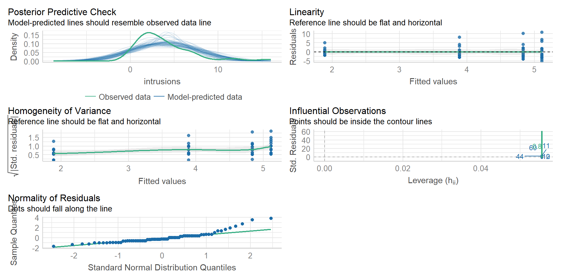
Checking the Assumptions

# "manually" check normality of residuals 

qqPlot(mod$aov$residuals)

[1]  3 57

shapiro.test(mod$aov$residuals)

    Shapiro-Wilk normality test

data:  mod$aov$residuals
W = 0.87739, p-value = 4.252e-06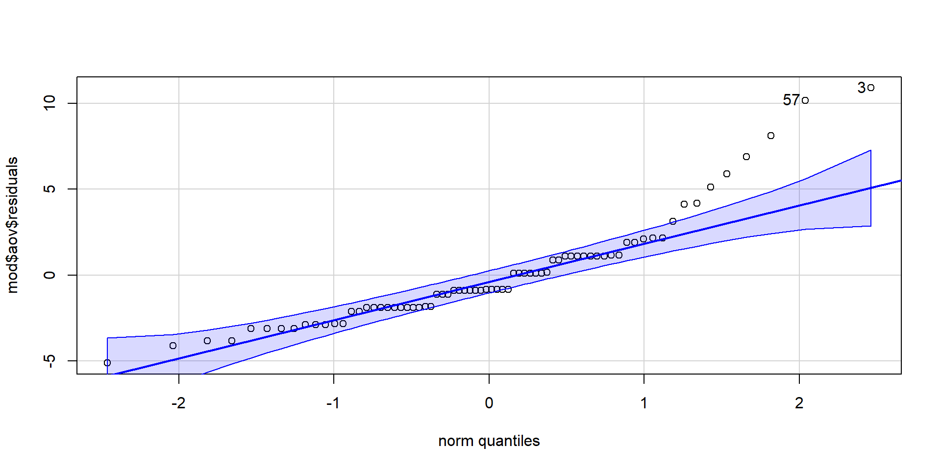

Checking the Assumptions

# check homogeneity of variance
test_levene(mod)

Warning: Variances differ between groups (Levene's Test, p = 0.039).

Both assumptions are not met!

But ANOVAS are quite robust to (minor) deviations…

If the assumptions are violated more, you could…
- run a non-parametric test (Kruskall-Wallis for between-subjects designs or Friedman for repeated measures)
- transform the data (see Field et al., 2009)
- use bootstrapping (see Field et al., 2009)

Post-Hoc Tests

So now we know that there are differences between the Conditions, but we don’t know yet which groups differ from each other. We could thus calculate pairwise comparisons or post-hoc t-tests to compare each condition to the others by filtering the data (so that only two conditions remain) and running t-tests.

A more convenient way is to use the emmeans() function from the package with the same name. We can also adjust the tests for multiple comparisons directly.

We could also define specific contrasts to test a priori (i.e., based on hypotheses). But we will skip this here.

Post-Hoc Tests

library(emmeans)
mod %>% emmeans(pairwise ~ Condition, adjust = "bonferroni") # also works with mod1!

$emmeans
 Condition emmean    SE df lower.CL upper.CL
 1           5.11 0.749 68    3.617     6.60
 2           1.89 0.749 68    0.395     3.38
 3           3.89 0.749 68    2.395     5.38
 4           4.83 0.749 68    3.340     6.33

Confidence level used: 0.95 

$contrasts
 contrast                estimate   SE df t.ratio p.value
 Condition1 - Condition2    3.222 1.06 68   3.044  0.0199
 Condition1 - Condition3    1.222 1.06 68   1.155  1.0000
 Condition1 - Condition4    0.278 1.06 68   0.262  1.0000
 Condition2 - Condition3   -2.000 1.06 68  -1.889  0.3787
 Condition2 - Condition4   -2.944 1.06 68  -2.781  0.0420
 Condition3 - Condition4   -0.944 1.06 68  -0.892  1.0000

P value adjustment: bonferroni method for 6 tests 

Should we adjust for multiple comparisons? It depends. There are good reasons for either.

ANOVA: Effect Sizes

The most common effect size estimate for an ANOVA is partial eta squared \(\eta_p^2\) (as we calculated with afex::aov_ez before). We get one per factor and it summarizes all pairwise effects within it.

We could also calculate Cohen’s d for each pairwise comparison within the factor but this is tedious and gets confusing quickly (1 factor with 5 levels = 10 effects; 3 factors with 5 levels each = 30 effects). It’s still sad that emmeans doesn’t output it as one additional column.

ANOVA: Power

Effect sizes are important to calculate the statistical power of your study before conducting it. Use an estimated effect size based on prior research:

library(pwr)
pwr.anova.test(k = 4, f = .4, sig.level = .05, power = .8) #we leave out the n parameter to let it be calculated

     Balanced one-way analysis of variance power calculation 

              k = 4
              n = 18.04262
              f = 0.4
      sig.level = 0.05
          power = 0.8

NOTE: n is number in each group

Note: f is “Cohen’s f”. You can convert your \(\eta_p^2\) to (partial) f using effectsize package:

effectsize::eta2_to_f(.15)

[1] 0.420084

Write Up

Once again, the apa package helps us here - if we used afex::aov_ez instead of lm 😅:

mod %>% apa::anova_apa()

       Effect                                              
1 (Intercept) F(1, 68) = 110.29, p < .001, petasq = .62 ***
2   Condition F(3, 68) =   3.79, p = .014, petasq = .14 *  

mod %>% emmeans("Condition") %>% pairs(adjust="none") #follow up t-tests without adjustment

 contrast                estimate   SE df t.ratio p.value
 Condition1 - Condition2    3.222 1.06 68   3.044  0.0033
 Condition1 - Condition3    1.222 1.06 68   1.155  0.2523
 Condition1 - Condition4    0.278 1.06 68   0.262  0.7938
 Condition2 - Condition3   -2.000 1.06 68  -1.889  0.0631
 Condition2 - Condition4   -2.944 1.06 68  -2.781  0.0070
 Condition3 - Condition4   -0.944 1.06 68  -0.892  0.3755

Looking at contrasts including condition 1 (control group): Only condition 2 different.
Let’s get the associated effect size of this specific contrast:

library(lsr)
cohensD(intrusions ~ Condition, 
        data = filter(dat, Condition %in% c(1,2)) %>% droplevels())

[1] 0.9964172

Write Up

       Effect                                              
1 (Intercept) F(1, 68) = 110.29, p < .001, petasq = .62 ***
2   Condition F(3, 68) =   3.79, p = .014, petasq = .14 *  

 contrast                estimate   SE df t.ratio p.value
 Condition1 - Condition2    3.222 1.06 68   3.044  0.0033
 Condition1 - Condition3    1.222 1.06 68   1.155  0.2523
 Condition1 - Condition4    0.278 1.06 68   0.262  0.7938
 Condition2 - Condition3   -2.000 1.06 68  -1.889  0.0631
 Condition2 - Condition4   -2.944 1.06 68  -2.781  0.0070
 Condition3 - Condition4   -0.944 1.06 68  -0.892  0.3755

[1] 0.9964172

There was a significant difference between groups in overall intrusion frequency in daily life, \(F(3, 68) = 3.79, p = 0.014, \eta_p^2 = .14\). Pairwise comparisons demonstrated that relative to the no-task control group, only those in the reactivation-plus-Tetris group, \(t(68) = 3.04, p < 0.01, d = 1.00\), experienced significantly fewer intrusive memories…

Thanks!

Learning objectives:

• Be able to run the following tests in R, check their assumptions, and report the results: Chi², t-tests, correlation, and one-way ANOVA

Next:

• General Linear Model!